Probabilistic Artificial Intelligence - Variational Inference

Variational Inference

The fundamental idea behind variational inference is to approximate the true posterior distribution using a “simpler” posterior that is as close as possible to the true posterior.

$$p(\theta\mid x_{1:n},y_{1:n})=\frac1Zp(\theta,y_{1:n}\mid x_{1:n})\approx q(\theta\mid\lambda)\doteq q_{\lambda}(\theta)$$

where λ represents the parameters of the variational posterior q, also called variational parameters.

Laplace Approximation

A natural idea for approximating the posterior distribution is to use a Gaussian approximation (that is, a second-order Taylor approximation) around the mode of the posterior. Such an approximation is known as a Laplace approximation.

As an example, we will look at Laplace approximation in the context of Bayesian logistic regression. Bayesian logistic regression corresponds to Bayesian linear regression with a Bernoulli likelihood.

Intuitively, the Laplace approximation matches the shape of the true posterior around its mode but may not represent it accurately elsewhere — often leading to extremely overconfident predictions.

Inference with a Variational

$$\begin{aligned} p(y^{\star}\mid x^{\star},x_{1:n},y_{1:n})& =\int p(y^\star\mid x^\star,\boldsymbol{\theta})p(\boldsymbol{\theta}\mid x_{1:n},y_{1:n})d\boldsymbol{\theta} \\ &\approx\int p(y^\star\mid x^\star,\boldsymbol{\theta})q_\lambda(\boldsymbol{\theta})d\boldsymbol{\theta} &=\int\int p(y^\star\mid f^\star)p(f^\star\mid x^\star,\theta)q_\lambda(\theta)d\theta df^\star\\&=\int p(y^\star\mid f^\star)\int p(f^\star\mid x^\star,\theta)q_\lambda(\theta)d\theta df^\star\\&=\int p(y^\star\mid f^\star)q_\lambda(f^\star\mid x^\star)df^\star.\quad\quad \end{aligned}$$

Information Theory

Surprise

The surprise about an event with probability u is defined as $S[u] = -log u$.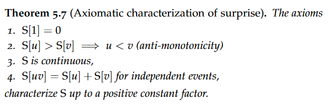

Entropy

The entropy of a distribution p is the average surprise about samples from p.if the entropy of p is large, we are more uncertain about x ∼ p than if the entropy of p were low.

$$\mathbb{H}[p]\doteq\mathbb{E}_{x\sim p}[\mathbb{S}[p(x)]]=\mathbb{E}_{x\sim p}[-\log p(x)].$$

Cross-Entropy

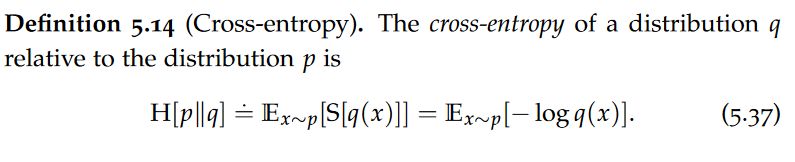
Cross-entropy can also be expressed in terms of the KL-divergence. Quite intuitively, the average surprise in samples from p with respect to the distribution q is given by the inherent uncertainty in p and the additional surprise that is due to us assuming the wrong data distribution q. The “closer” q is to the true data distribution p, the smaller is the additional average surprise.

$$\mathrm{H}[p\|q]=\mathrm{H}[p]+\mathrm{KL}(p\|q)\geq\mathrm{H}[p].$$

Variational Families

We can view variational inference more generally as a family of approaches aiming to approximate the true posterior distribution by one that is closest (according to some criterion) among a “simpler” class of distributions.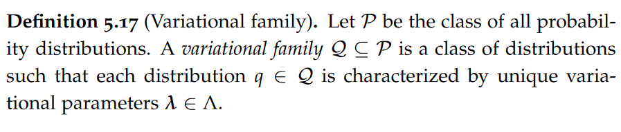

Kullback-Leibler Divergence

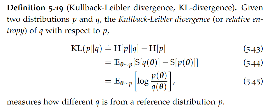
In words, KL(p∥q) measures the additional expected surprise when observing samples from p that is due to assuming the (wrong) distribution q and which not inherent in the distribution p already. Intuitively, the KL-divergence measures the information loss when approximating p with q.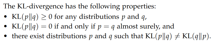

Forward and reverse KL-divergence

KL(p∥q) is also called the forward (or inclusive) KL-divergence. In contrast, KL(q∥p) is called the reverse (or exclusive) KL-divergence.

It can be seen that the reverse KL-divergence tends to greedily select the mode and underestimating the variance which, in this case, leads to an overconfident prediction. The forward KL-divergence, in contrast, is more conservative and yields what one could consider the “desired” approximation.

The reverse KL-divergence is typically used in practice. This is for computational reasons. In principle, if the variational family Q is “rich enough”, minimizing the forward and reverse KL-divergences will yield the same result.

There is a nice interpretation of minimizing the forward KullbackLeibler divergence of the approximation $q_\lambda$ with respect to the true distribution p as being equivalent to maximizing the marginal model likelihood on a sample of infinite size. This interpretation is not useful in the setting where p is a posterior distribution over model parameters θ as a maximum likelihood estimate requires samples from p which we cannot obtain in this case.

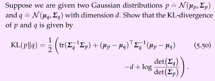
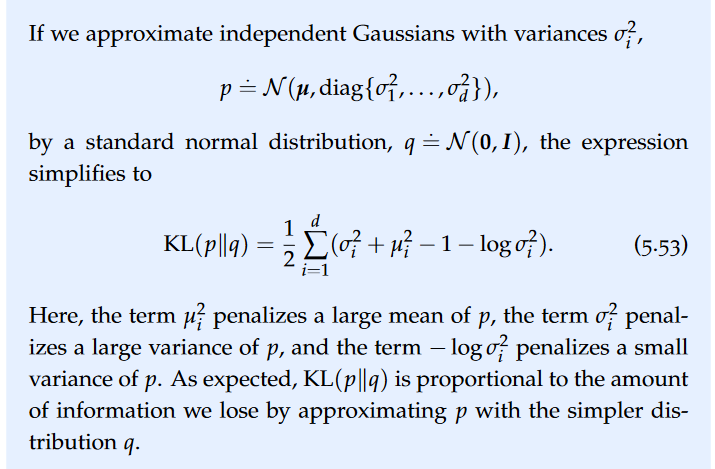
KL-divergence of Gaussians

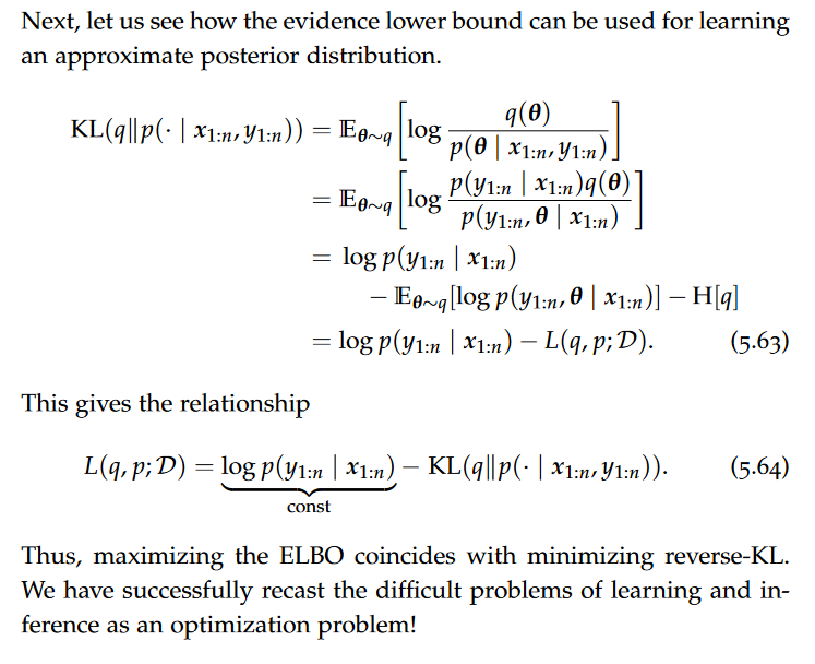
Evidence Lower Bound

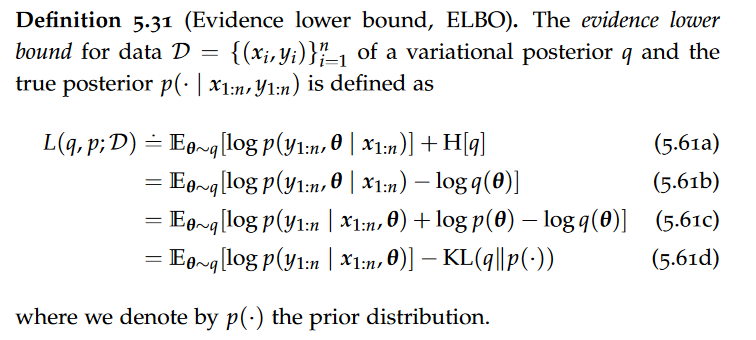
The Evidence Lower Bound is a quantity maximization of which is equivalent to minimizing the KL-divergence. As its name suggests, the evidence lower bound is a (uniform) lower bound to the log-evidence $log p(y{1:n}|x{1:n})$.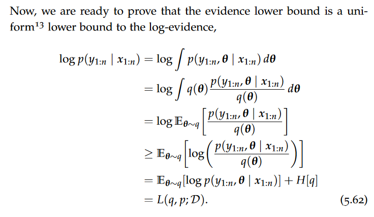

Note that this inequality lower bounds the logarithm of an integral by an expectation of a logarithm over some variational distribution q. Hence, the ELBO is a family of lower bounds — one for each variational distribution. Such inequalities are called variational inequalities.

Gradient of Evidence Lower Bound

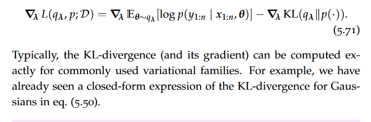
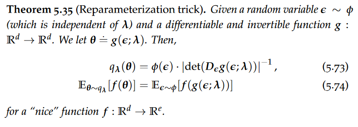
Obtaining the gradient of the evidence lower bound is more difficult. This is because the expectation integrates over the measure $q_\lambda$, which depends on the variational parameters $\lambda$. Thus, we cannot move the gradient operator inside the expectation.

There are two main techniques which are used to rewrite the gradient in such a way that Monte Carlo sampling becomes possible. The first is to use score gradients. The second is the so-called reparameterization trick.

reparameterization trick

The procedure of approximating the true posterior using a variational posterior by maximizing the evidence lower bound using stochastic optimization is also called black box stochastic variational inference. The only requirement is that we can obtain unbiased gradient estimates from the evidence lower bound (and the likelihood).