pai - Bayesian Optimization

Bayesian Optimization

Exploration-Exploitation Dilemma

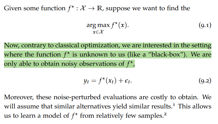
In Bayesian optimization, we want to learn a model of f ⋆ and use this model to optimize f ⋆ simultaneously. These goals are somewhat contrary. Learning a model of f ⋆ requires us to explore the input space while using the model to optimize f ⋆ requires us to focus on the most promising well-explored areas. This trade-off is commonly known as the exploration-exploitation dilemma.

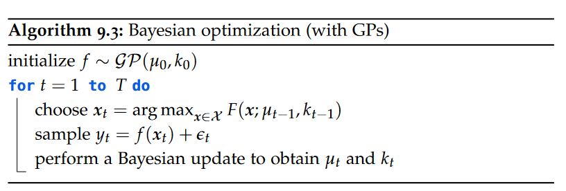
It is common to use a so-called acquisition function to greedily pick the next point to sample based on the current model.

Online Learning and Bandits

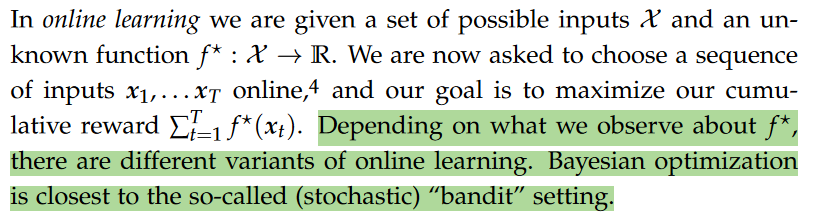
Multi-Armed Bandits(MAB)

The “multi-armed bandits” (MAB) problem is a classical, canonical formalization of the exploration-exploitation dilemma. In the MAB problem, we are provided with k possible actions (arms) and want to maximize our reward online within the time horizon T. We do not know the reward distributions of the actions in advance, however, so we need to trade learning the reward distribution with following the most promising action.

Bayesian optimization can be interpreted as a variant of the MAB problem where there can be a potentially infinite number of actions (arms), but their rewards are correlated (because of the smoothness of the Gaussian process prior). Smoothness means that nearby points in the input space are likely to have similar function values. Because of the smoothness property inherent in the Gaussian process prior, Bayesian optimization can make informed decisions about where to explore next in the input space. The model can leverage information from previously evaluated points to predict the behavior of the objective function at unexplored points more effectively.

Regret

The key performance metric in online learning is the regret.

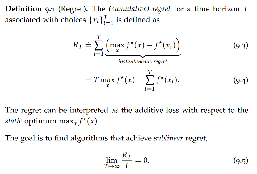
Achieving sublinear regret requires balancing exploration with exploitation. Typically, online learning (and Bayesian optimization) consider stationary environments, hence the comparison to the static optimum.

Acquisition Functions

Throughout our description of acquisition functions, we will focus on a setting where we model $f^⋆$ using a Gaussian process which we denote by f. The methods generalize to other means of learning $f^⋆$ such as Bayesian neural networks.

One possible acquisition function is uncertainty sampling. However, this acquisition function does not at all take into account the objective of maximizing $f^⋆$ and focuses solely on exploration.

Suppose that our model f of $f^⋆$ is well-calibrated, in the sense that the true function lies within its confidence bounds. Consider the best lower bound, that is, the maximum of the lower confidence bound. Now, if the true function is really contained in the confidence bounds, it must hold that the optimum is somewhere above this best lower bound.

Therefore, we only really care how the function looks like in the regions where the upper confidence bound is larger than the best lower bound. The key idea behind the methods that we will explore is to focus exploration on these plausible maximizers.

Upper Confidence Bound

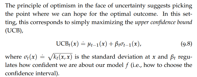
This acquisition function naturally trades exploitation by preferring a large posterior mean with exploration by preferring a large posterior variance.
This optimization problem is non-convex in general. However, we can use approximate global optimization techniques like Lipschitz optimization (in low dimensions) and gradient ascent with random initialization (in high dimensions). Another widely used option is to sample some random points from the domain, score them according to this criterion, and simply take the best one.

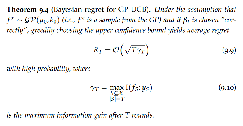
Observe that if the information gain is sublinear in T then we achieve sublinear regret and, in particular, converge to the true optimum. The term “sublinear” refers to a growth rate that is slower than linear.

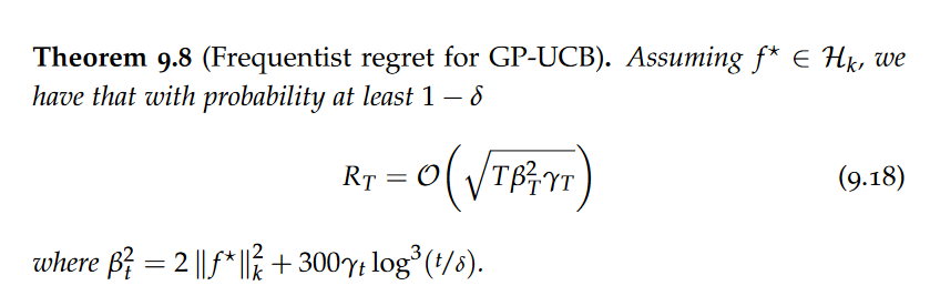
Intuitively, to work even if the unknown function $f^⋆$ is not contained in the confidence bounds, we use βt to re-scale the confidence bounds to enclose $f^⋆$.

Probability of Improvement

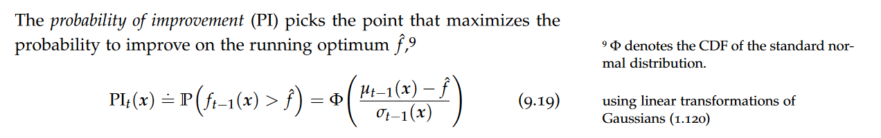
Probability of improvement tends to be biased in favor of exploitation, as it prefers points with large posterior mean and small posterior variance.

Expected Improvement

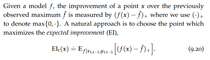
Intuitively, expected improvement seeks a large expected improvement (exploitation) while also preferring states with a large variance (exploration).

Thompson Sampling

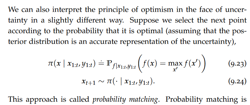
Probability matching is exploratory as it prefers points with larger variance (as they automatically have a larger chance of being optimal), but at the same time exploitative as it effectively discards points with low posterior mean and low posterior variance. Unfortunately, it is generally difficult to compute π analytically given a posterior. Instead, it is common to use a sampling-based approximation of π.

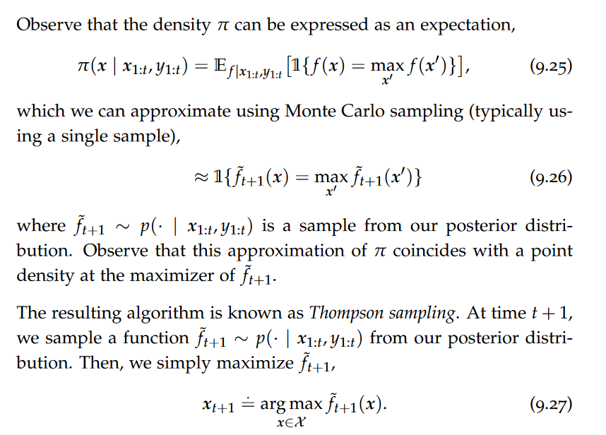
In many cases, the randomness in the realizations of ̃ ft+1 is already sufficient to effectively trade exploration and exploitation.

Model Selection

Selecting a model of f ⋆ is much harder than in the i.i.d. data setting of supervised learning. There are mainly the two following dangers, • the data sets collected in active learning and Bayesian optimization are small; and • the data points are selected dependently on prior observations. This leads to a specific danger of overfitting. In particular, due to feedback loops between the model and the acquisition function, one may end up sampling the same point repeatedly.

Another approach that often works fairly well is to occasionally (according to some schedule) select points uniformly at random instead of using the acquisition function. This tends to prevent getting stuck in suboptimal parts of the state space.

difference betwwen active learning and Bayesian Optimization

Problem Setting:
Active Learning: Active learning typically deals with supervised learning tasks where there is a large pool of unlabeled instances, and the algorithm decides which instances to query for labels to improve the model.
Bayesian Optimization: Bayesian optimization deals with optimization problems where the objective function is unknown, expensive to evaluate, and possibly noisy. It aims to find the global optimum with as few evaluations as possible.

Nature of Queries:
Active Learning: In active learning, the queries are often in the form of “Which instance should be labeled next?” The goal is to select instances that will most benefit the model’s learning process.
Bayesian Optimization: In Bayesian optimization, the queries are in the form of “What point should be evaluated next in the input space to maximize/minimize the objective function?” The goal is to efficiently explore the input space and find the optimal configuration.

Algorithmic Approaches:
Active Learning: Active learning involves various strategies such as uncertainty sampling, query-by-committee, and diversity sampling to select informative instances for labeling.
Bayesian Optimization: Bayesian optimization employs probabilistic surrogate models (often Gaussian processes) to model the unknown objective function. Acquisition functions guide the search to balance exploration and exploitation efficiently.