fundamentals

probability

sample space, event space, σ-algebra and probability space

A probability space is a mathematical construct that consists of three elements: the sample space (S), the event space (E), and a probability measure (P). Additionally, a sigma-algebra (σ-algebra) is associated with the event space.

The sample space is the set of all possible outcomes of an experiment.The event space is a collection of subsets of the sample space.
A sigma-algebra is a collection of subsets of the sample space. It includes the sample space, is closed under complementation, and is closed under countable unions. The probability measure is a function that assigns probabilities to events.

probability mass function (PMF) and cumulative distribution function (CDF),probability density function (PDF)

The Probability Mass Function (PMF) is a function that gives the probability that a discrete random variable is exactly equal to a certain value. The Cumulative Distribution Function (CDF) of a random variable gives the probability that
X takes on a value less than or equal to x.
The Probability Density Function (PDF) is applicable to continuous random variables.The total area under the PDF curve is equal to 1.

Continuous Distributions

normal distribution(Gaussian):The Gaussian CDF cannot be expressed in closed-form. Note that the mean of a Gaussian distribution coincides with the maximizer of its PDF, also called mode of a distribution.

Joint Probability, Conditional Probability, Sum rule, Product rule(chain rule),the law of total probability

Joint probability refers to the probability of the occurrence of two or more events simultaneously. Conditional probability is the probability of one event occurring given that another event has already occurred. The sum rule, or addition rule, gives the probability of the union of two events. The product rule, also known as the chain rule, provides a way to express the joint probability of multiple events. The law of total probability is a way to express the probability of an event B by considering all possible ways in which
B can occur.

independence, conditional independence

Conditional independence does not necessarily imply unconditional independence, and vice versa.

Directed Graphical Models(Bayesian networks)

Directed graphical models (also called Bayesian networks) are often used to visually denote the (conditional) independence relationships of a large number of random variables.

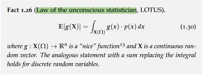
Expectation, Covariance and Variance, Standard deviation,Law of total variance

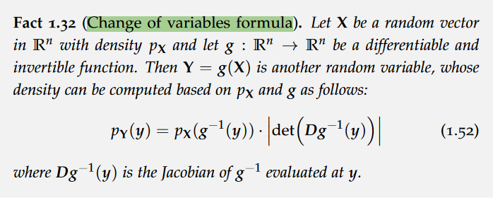
Change of variables formula

Probabilistic inference

Bayes’ rule,Conjugate Priors

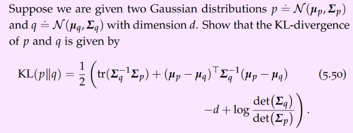
gaussian,Guassian random vector

Any affine transformation of a Gaussian random vector is a Gaussian random vector.

Supervised Learning and Point Estimates

Maximum Likelihood Estimation,Maximum a Posteriori Estimation,

The MLE and MAP estimate can be seen as a naïve approximation of probabilistic inference, represented by a point density which “collapses” all probability mass at the mode of the posterior distribution.

exercise

affine transformation,Jacobian matrix,

PML

linear regression

linear regression(MLE), ridge regression(MAP)

ridge,lasso

least absolute shrinkage and selection operator (lasso): Laplace prior, L1 regularization.
Ridge: Gaussian prior, L2 regularization.

The primary difference lies in the penalty terms: L1 regularization uses the sum of absolute values, and L2 regularization uses the sum of squared values.
L1 regularization tends to result in exact zeros, leading to sparse solutions, whereas L2 regularization generally leads to smaller, non-zero coefficients.

Bayesian linear regression (BLR)

Aleatoric and Epistemic Uncertainty

epistemic uncertainty: corresponds to the uncertainty about our model due to the lack of data. aleatoric uncertainty: “irreducible noise”, cannot be explained by the inputs and any model from the model class.

equation under the law of total variance.

kernel

Filtering

The process of keeping track of the state using noisy observations is also known as Bayesian filtering or recursive Bayesian estimation.

Kalman filter

A Kalman filter is simply a Bayes filter using a Gaussian distribution over the states and conditional linear Gaussians to describe the evolution of states and observations.

Gaussian Process

A Gaussian process is an infinite set of random variables such that any finite number of them are jointly Gaussian.

kernel function, feature space, RKHS,Stationarity and isotropy

A Gaussian process with a linear kernel is equivalent to Bayesian linear regression.

For ν = 1/2, the Matérn kernel is equivalent to the Laplace kernel. For ν → ∞, the Matérn kernel is equivalent to the Gaussian kernel.

Note that stationarity is a necessary condition for isotropy. In other words, isotropy implies stationarity.

skip 4.3.4

model selection

Maximizing the Marginal Likelihood

Marginal likelihood maximization is an empirical Bayes method. Often it is simply referred to as empirical Bayes.
this approach typically avoids overfitting even though we do not use a separate training and validation set. maximizing the marginal likelihood naturally encourages trading between a large likelihood and a large prior.

Approximations

random Fourier features,Bochner’s theorem,Uniform convergence of Fourier features

inducing points method,subset of regressors (SoR) approximation,fully independent training conditional (FITC) approximation

Variational Inference

Laplace Approximation,Bayesian Logistic Regression,

The Laplace approximation matches the shape of the true posterior around its mode but may not represent it accurately elsewhere — often leading to extremely overconfident predictions.

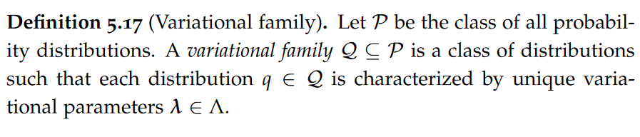
Variational family,mean-field distribution

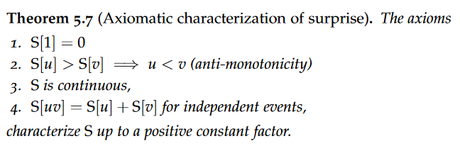
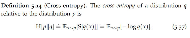
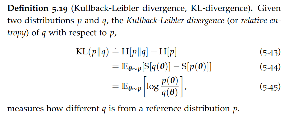
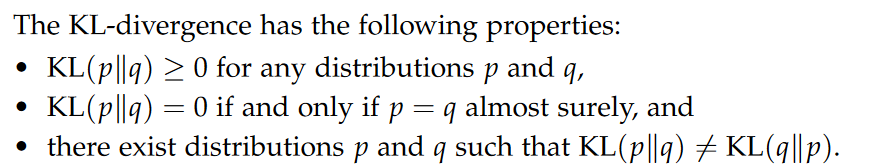
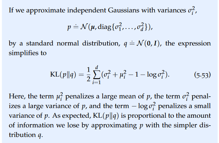
Information Theory,Surprise,entropy,Jensen’s Inequality,Cross-entropy,KL-divergence,Forward and Reverse KL-divergence

The uniform distribution has the maximum entropy among all discrete distributions supported on {1, . . . , n}.

In words, KL(p∥q) measures the additional expected surprise when observing samples from p that is due to assuming the (wrong) distribution q.

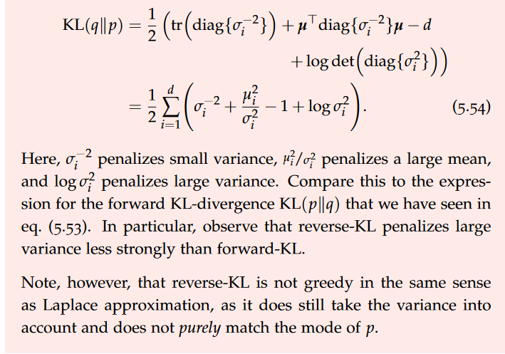
It can be seen that the reverse KL-divergence tends to greedily select the mode and underestimating the variance which, in this case, leads to an overconfident prediction. The forward KL-divergence, in contrast, is more conservative.

Note, however, that reverse-KL is not greedy in the same sense as Laplace approximation, as it does still take the variance into account and does not purely match the mode of p.

Minimizing Forward-KL as Maximum Likelihood Estimation,Minimizing Forward-KL as Moment Matching

First, we observe that minimizing the forward KL-divergence is equivalent to maximum likelihood estimation on an infinitely large sample size.

A Gaussian qλ minimizing KL(p∥qλ) has the same first and second moment as p.

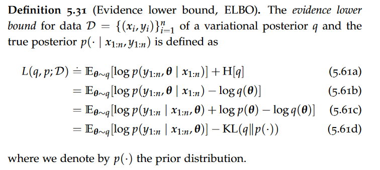
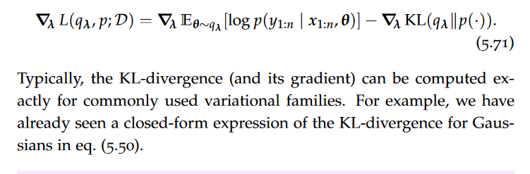
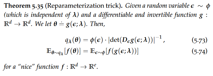
Evidence Lower Bound,Gaussian VI vs Laplace approximation, Gradient of Evidence Lower Bound(score gradients and Reparameterization trick)

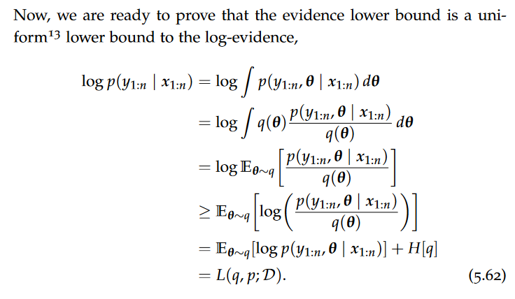
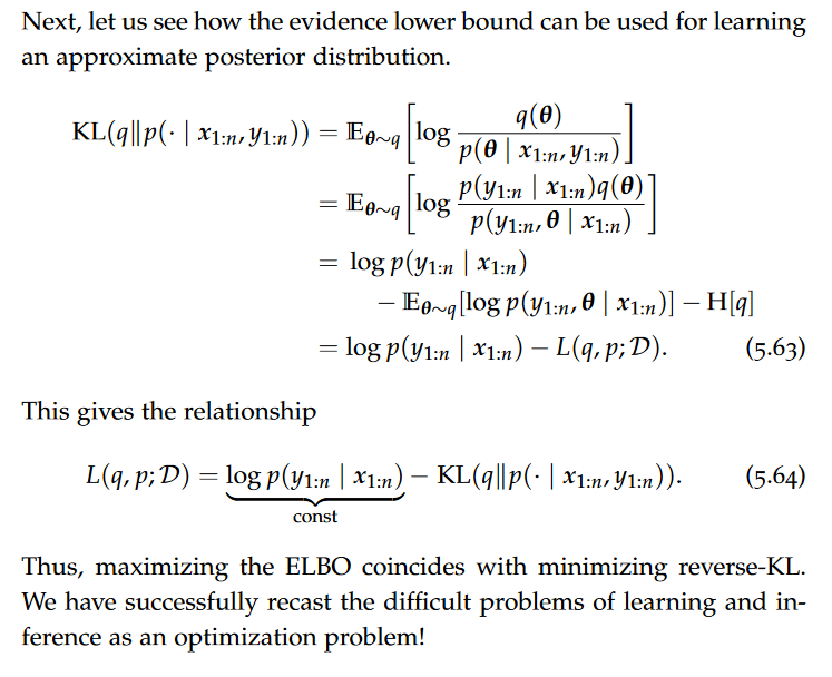
maximizing the ELBO coincides with minimizing reverse-KL.

maximizing the ELBO selects a variational distribution q that is close to the prior distribution p(·) while also maximizing the average likelihood of the data p(y1:n | x1:n, θ) for θ ∼ q.

Note that for a noninformative prior p(·) ∝ 1, maximizing the ELBO is equivalent to maximum likelihood estimation.

skip 5.5.2

Markov Chain Monte Carlo Methods

The key idea of Markov chain Monte Carlo methods is to construct a Markov chain, which is efficient to simulate and has the stationary distribution p.

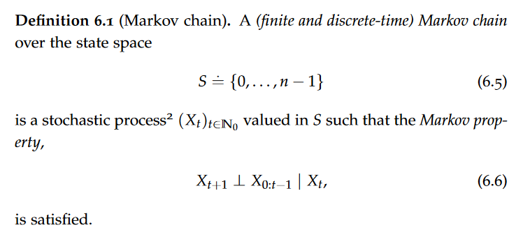
Markov Chains(Stationarity,convergence), Markov property,time-homogeneous Markov chains

Intuitively, the Markov property states that future behavior is independent of past states given the present state.

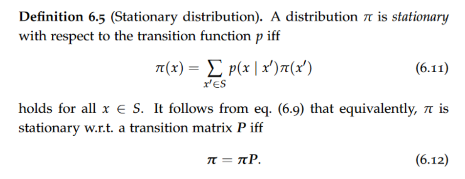
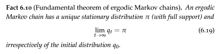
Stationary distribution,aperiodic,Ergodicity,Fundamental theorem of ergodic Markov chains

After entering a stationary distribution π, a Markov chain will always remain in the stationary distribution.

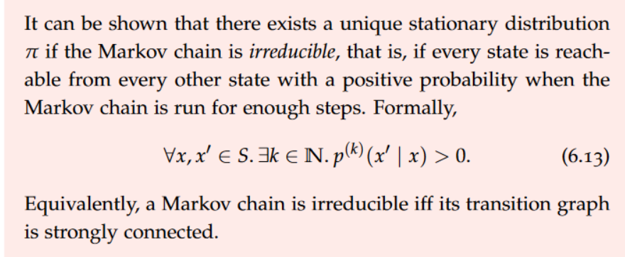
It can be shown that there exists a unique stationary distribution π if the Markov chain is irreducible, that is, if every state is reachable from every other state with a positive probability when the Markov chain is run for enough steps.

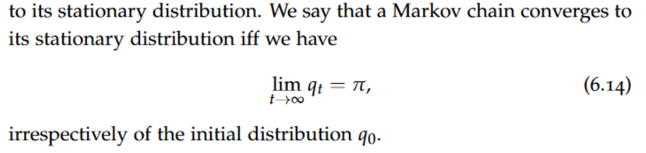
Even if a Markov chain has a unique stationary distribution, it must not converge to it.

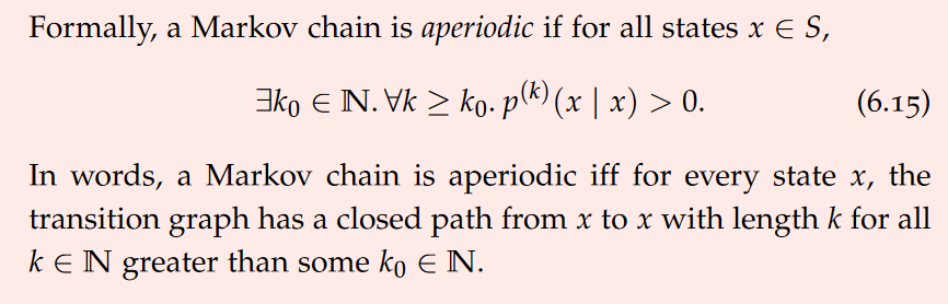
In words, a Markov chain is aperiodic iff for every state x, the transition graph has a closed path from x to x with length k for all k ∈ N greater than some k0 ∈ N.

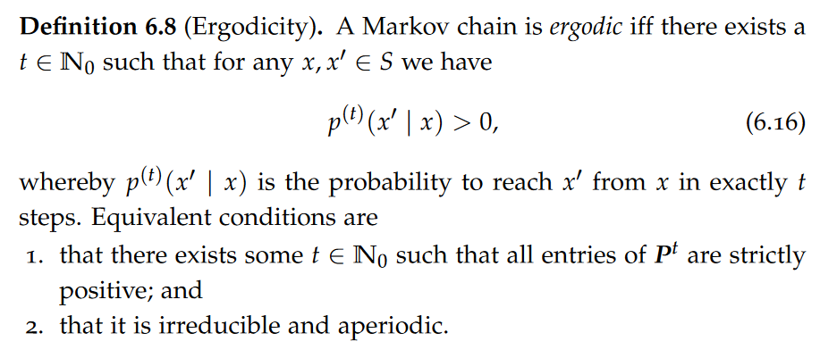
A Markov chain is ergodic iff there exists a t ∈ N0 such that for any x, x′ ∈ S we have p(t)(x′ | x) > 0.

A commonly used strategy to ensure that a Markov chain is ergodic is to add “self-loops” to every vertex in the transition graph.

An ergodic Markov chain has a unique stationary distribution π (with full support) irrespectively of the initial distribution q0. This naturally suggests constructing an ergodic Markov chain such that its stationary distribution coincides with the posterior distribution. If we then sample “sufficiently long”, Xt is drawn from a distribution that is “very close” to the posterior distribution.

How quickly does a Markov chain converge?(Total variation distance and Mixing time)

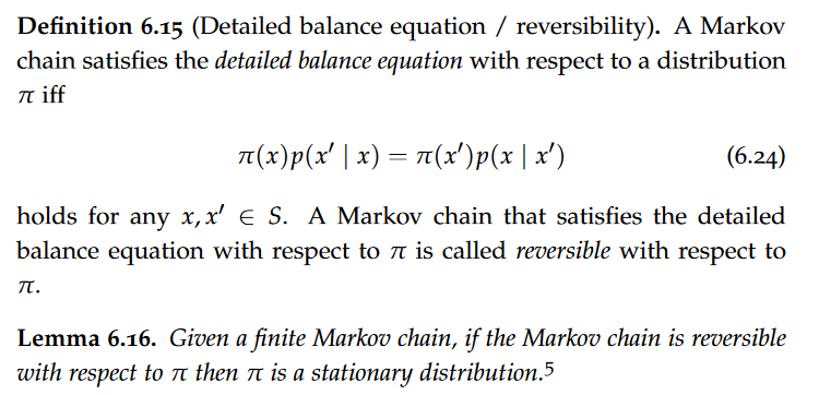
Detailed Balance Equation,Ergodic Theorem

A Markov chain that satisfies the detailed balance equation with respect to π is called reversible with respect to π.

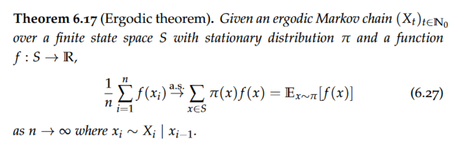
Ergodic Theorem is a way to generalize the (strong) law of large numbers to Markov chains.

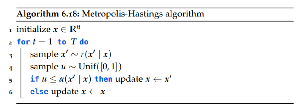
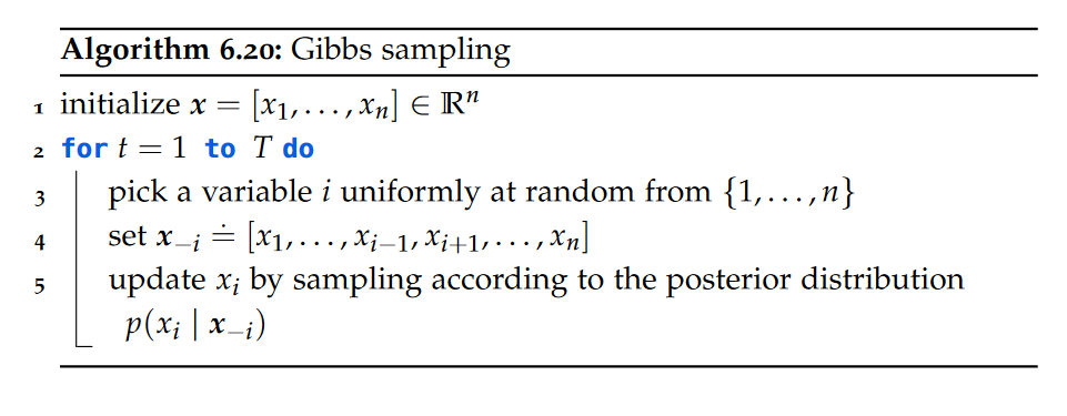
Elementary Sampling Methods,Metropolis-Hastings Algorithm,Metropolis-Hastings theorem, Gibbs Sampling

A popular example of a Metropolis-Hastings algorithm is Gibbs sampling.

Sampling as Optimization,Gibbs distribution,Langevin Dynamics,Metropolis adjusted Langevin algorithm (MALA) or Langevin Monte Carlo (LMC),unadjusted Langevin algorithm (ULA), Stochastic Gradient Langevin Dynamics, Hamiltonian Monte Carlo

A useful property is that Gibbs distributions always have full support. Observe that the posterior distribution can always be interpreted as a Gibbs distribution as long as prior and likelihood have full support.

Langevin dynamics adapts the Gaussian proposals of the Metropolis-Hastings algorithm to search the state space in an “informed” direction. The simple idea is to bias the sampling towards states with lower energy, thereby making it more likely that a proposal is accepted. A natural idea is to shift the proposal distribution perpendicularly to the gradient of the energy function. The resulting variant of Metropolis-Hastings is known as the Metropolis adjusted Langevin algorithm (MALA) or Langevin Monte Carlo (LMC).

The HMC algorithm is an instance of Metropolis-Hastings which uses momentum to propose distant points that conserve energy, with high acceptance probability.

path

target: show that the stationary distribution of a Markov chain coincides with the posterior distribution.
base: Detailed Balance Equation which shows that A Markov chain that satisfies the detailed balance equation with respect to π is called reversible with respect to π and if the Markov chain is reversible with respect to π then π is a stationary distribution. With posterior distribution p(x) = 1/Z q(x), substitute the posterior for π in the detailed balance equation, we can remove z, so we do not need to know the true posterior p to check that the stationary distribution of our Markov chain coincides with p, it suffices to know the finite measure q. However, until now, this does not allow us to estimate expectations over the posterior distribution. Note that although constructing such a Markov chain allows us to obtain samples from the posterior distribution, they are not independent. Thus, the law of large numbers and Hoeffding’s inequality do not apply, but there is a way to generalize the (strong) law of large numbers to Markov chains, which is Ergodic theorem.

Next we need to consider how to construct Markov chain with the goal of approximating samples from the posterior distribution p. One way is Metropolis-Hastings Algorithm, in which we are given a proposal distribution and we use the acceptance distribution to decide whether to follow the proposal. Another way is Gibbs sampling.

MCMC techniques can be generalized to
continuous random variables / vectors. Observe that the posterior distribution can always be interpreted as a Gibbs distribution as long as prior and likelihood have full support.

Langevin dynamics adapts the Gaussian proposals of the Metropolis-Hastings algorithm to search the state space in an “informed” direction. The simple idea is to bias the sampling towards states with lower energy, thereby making it more likely that a proposal is accepted. A natural idea is to shift the proposal distribution perpendicularly to the gradient of the energy function. The resulting variant of Metropolis-Hastings is known as the Metropolis adjusted Langevin algorithm (MALA) or Langevin Monte Carlo (LMC).

skip 6.3.5

BDL

Artificial Neural Networks,Activation Functions,

Non-linear activation functions allow the network to represent arbitrary functions. This is known as the universal approximation theorem.

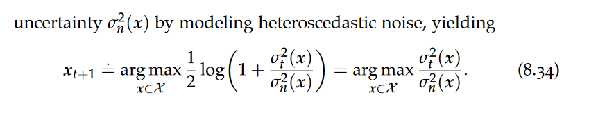
Bayesian Neural Networks, Heteroscedastic Noise, Variational Inference,Markov Chain Monte Carlo, SWA,SWAG,Dropout and Dropconnect, Probabilistic Ensembles

Intuitively, variational inference in Bayesian neural networks can be interpreted as averaging the predictions of multiple neural networks drawn according to the variational posterior qλ.

Calibration,expected calibration error (ECE), maximum calibration error (MCE), Histogram binning, Isotonic regression, Platt scaling, Temperature scaling

We say that a model is wellcalibrated if its confidence coincides with its accuracy across many predictions. Compare within each bin, how often the model thought the inputs belonged to the class (confidence) with how often the inputs actually belonged to the class (frequency).

Sequential Decision-Making

Active Learning

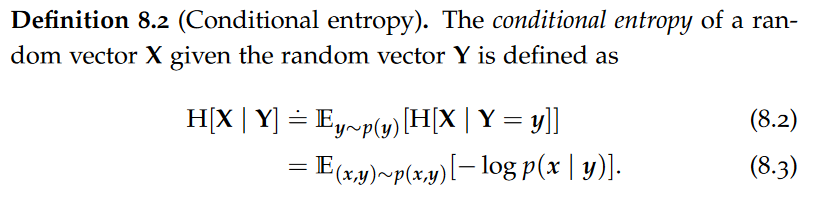
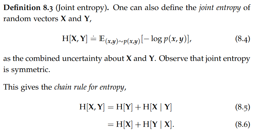
Conditional Entropy,Joint entropy

A very intuitive property of entropy is its monotonicity: when conditioning on additional observations the entropy can never increase.

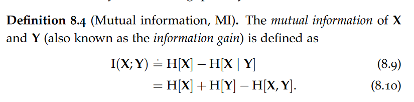
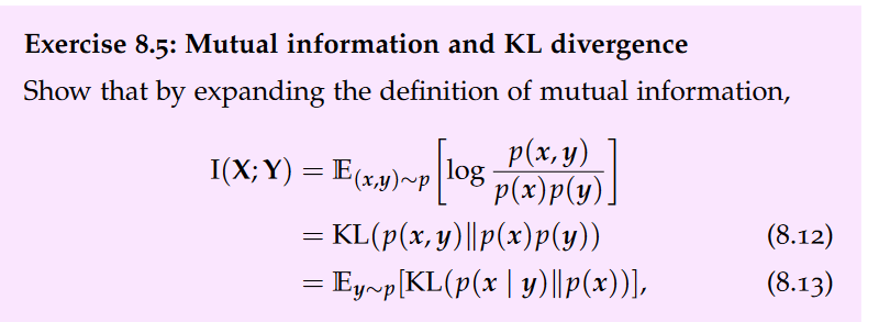
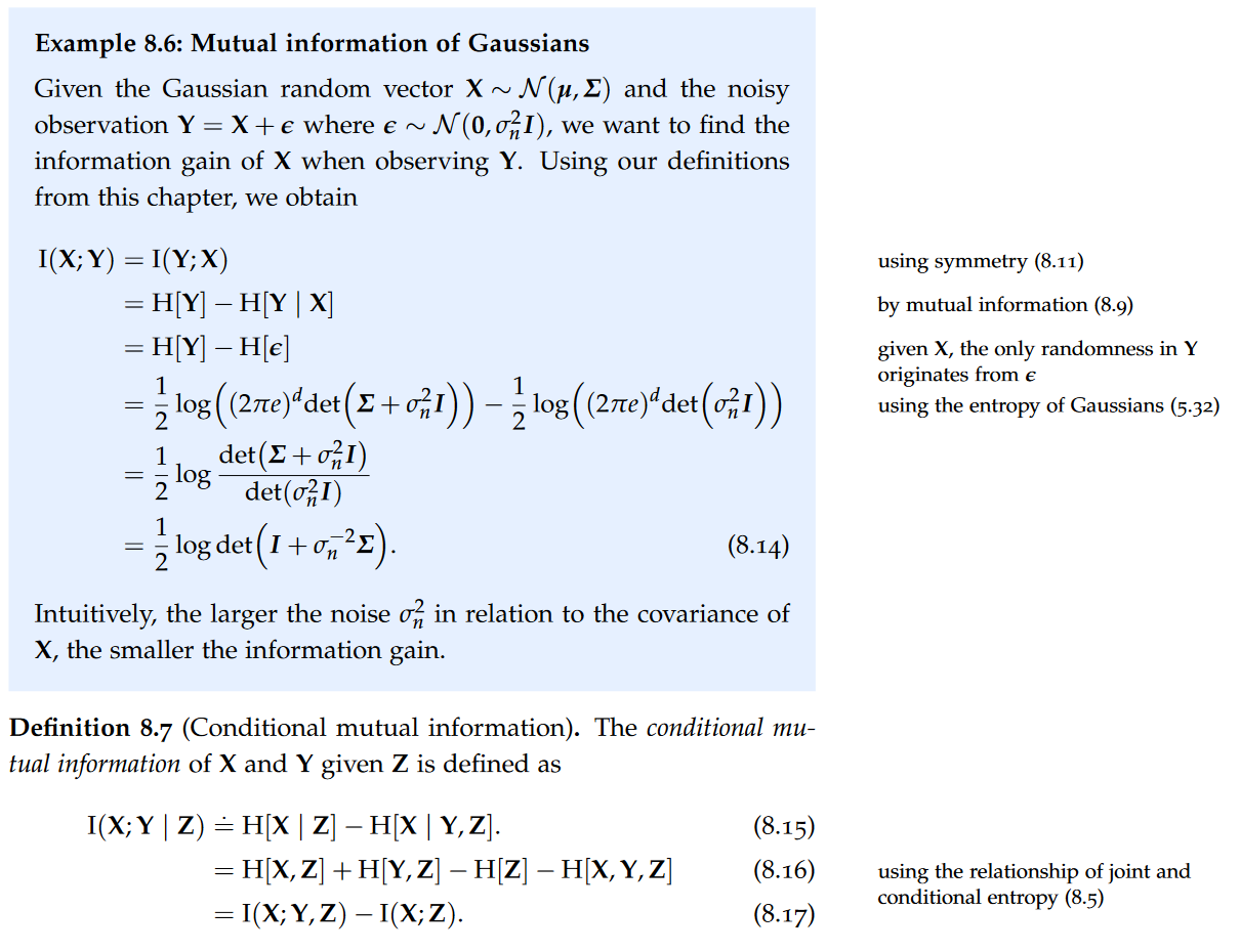
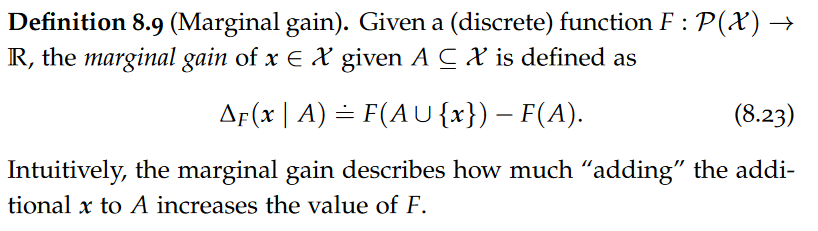
Mutual Information(information gain), the law of total expectation, data processing inequality, interaction information(Synergy and Redundancy), Submodularity of Mutual Information, Marginal gain, Submodularity, monotone,

data processing inequality: which says that processing cannot increase the information contained in a signal.

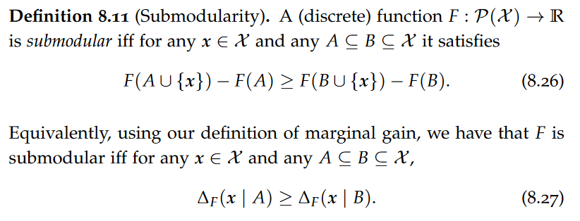
F is submodular iff “adding” x to the smaller set A yields more marginal gain than adding x to the larger set B.

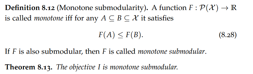
I is monotone submodular.

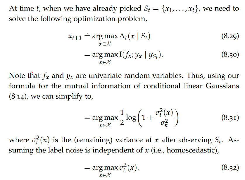
Maximizing Mutual Information, Greedy submodular function maximization, Uncertainty Sampling, Marginal gain of maximizing mutual information,Bayesian active learning by disagreement (BALD)

skip proof of Theorem 8.15

Therefore, if f is modeled by a Gaussian and we assume homoscedastic noise, greedily maximizing mutual information corresponds to simply picking the point x with the largest variance. This algorithm is also called uncertainty sampling.

Experimental Design, Entropy Search

skip

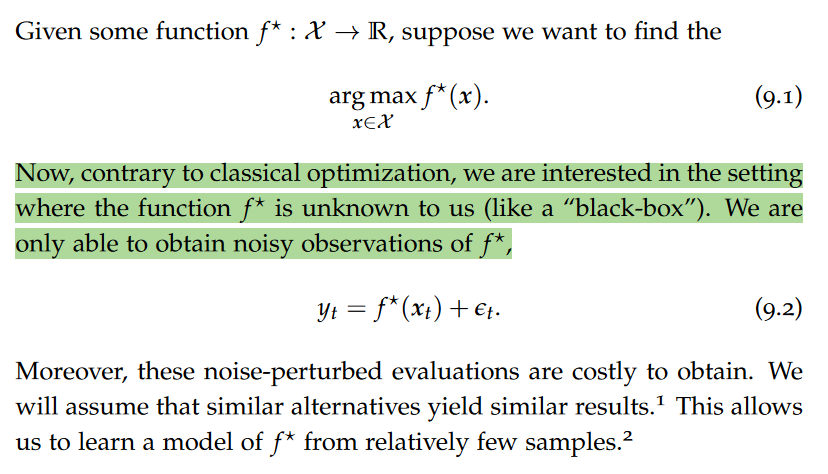
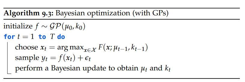
Bayesian Optimization

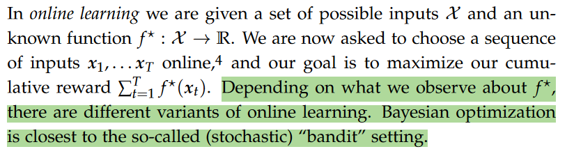
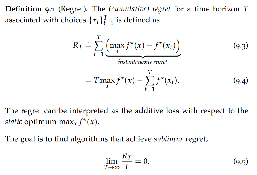
Exploration-Exploitation Dilemma,Online Learning and Bandits, Multi-Armed Bandits, Regret, sublinear regret, Cesàro mean

Bayesian optimization can be interpreted as a variant of the MAB problem where there can be a potentially infinite number of actions (arms), but their rewards are correlated (because of the smoothness of the Gaussian process prior).

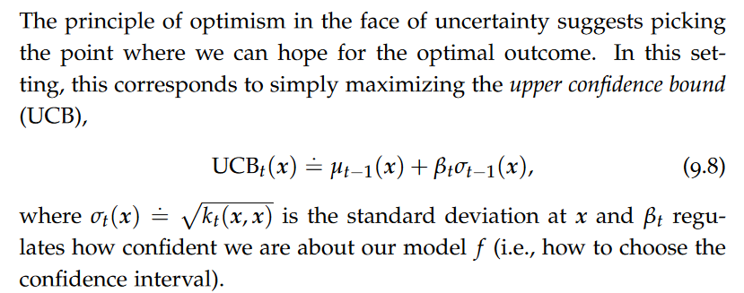
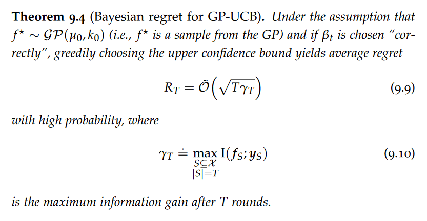
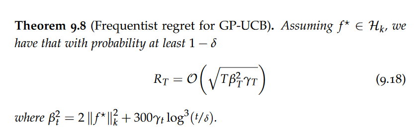
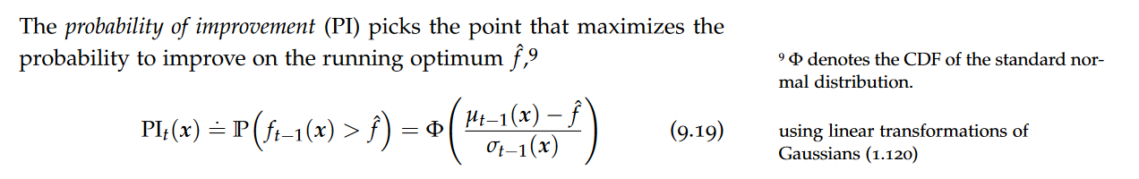
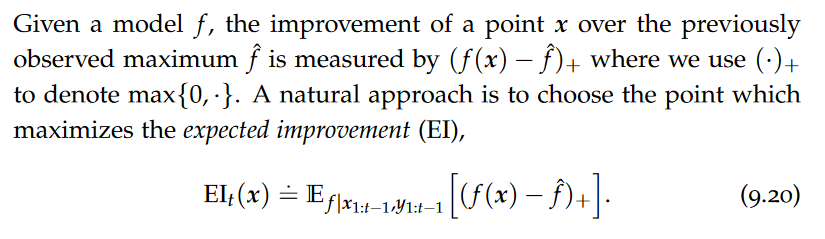
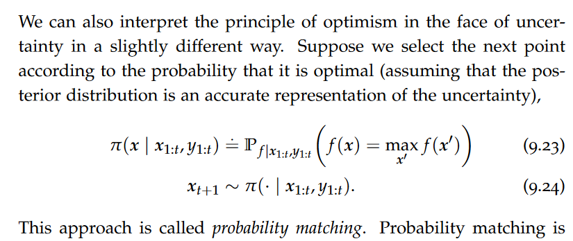
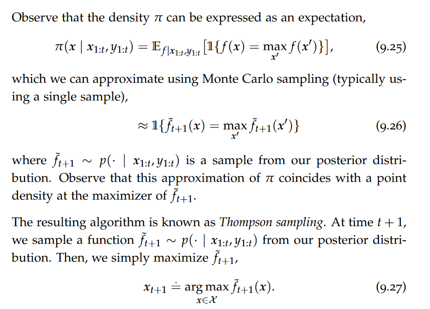
Acquisition Functions, Upper Confidence Bound, Bayesian confidence intervals, Regret of GP-UCB, Information gain of common kernels, Frequentist confidence intervals, probability of improvement, expected improvement (EI), Thompson Sampling, probability matching, Information-Directed Sampling

skip Information-Directed Sampling

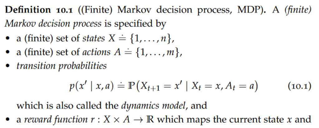
Markov Decision Processes

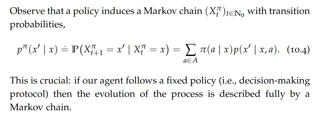
Planning deals with the problem of deciding which action an agent should play in a (stochastic) environment. A key formalism for probabilistic planning in known environments are so-called Markov decision processes.

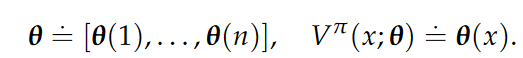
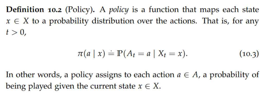
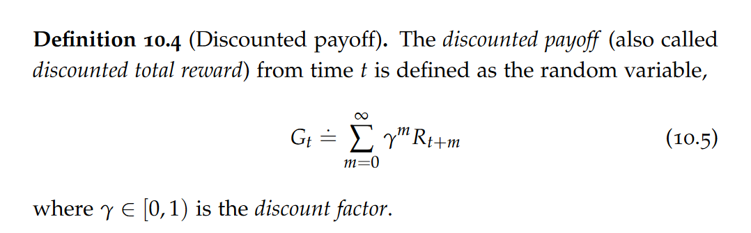
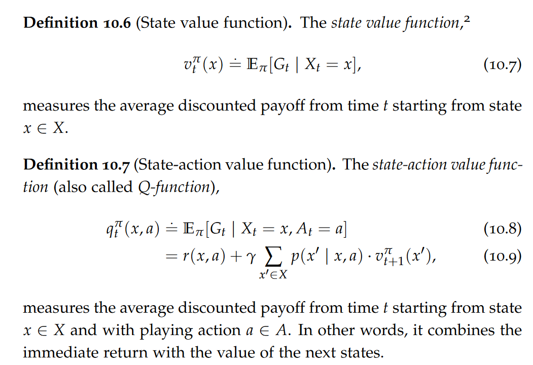
Policy,discounted payoff,state value function,state-action value function (also called Q-function)

A policy is a function that maps each state x ∈ X to a probability distribution over the actions.

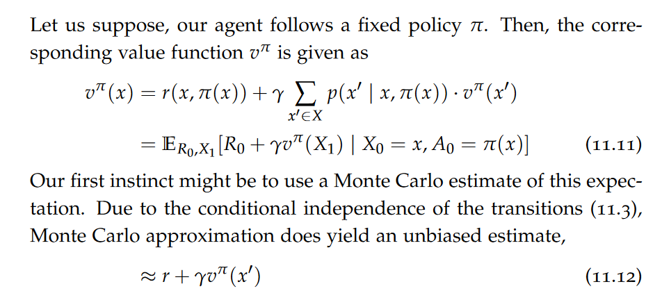
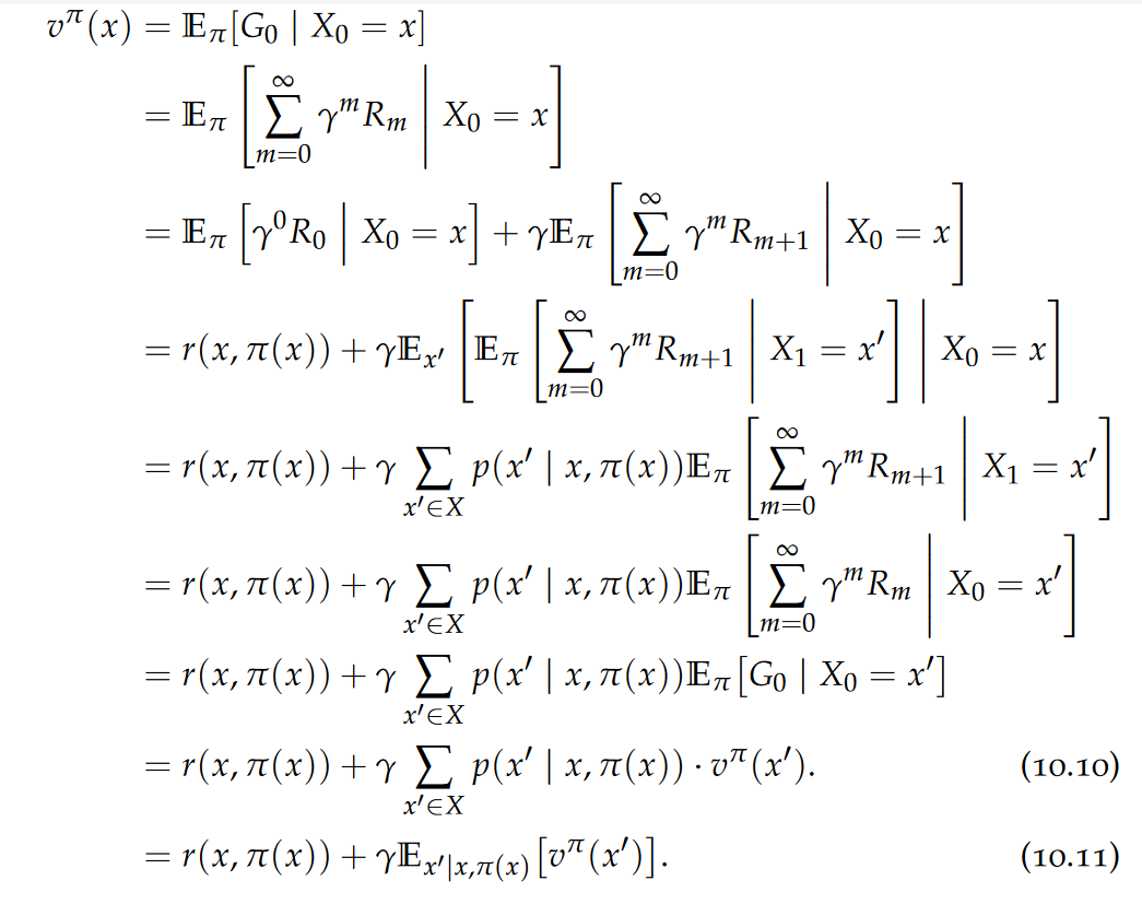
Bellman Expectation Equation

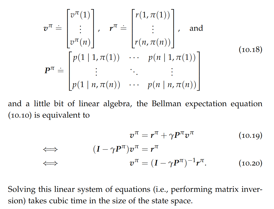
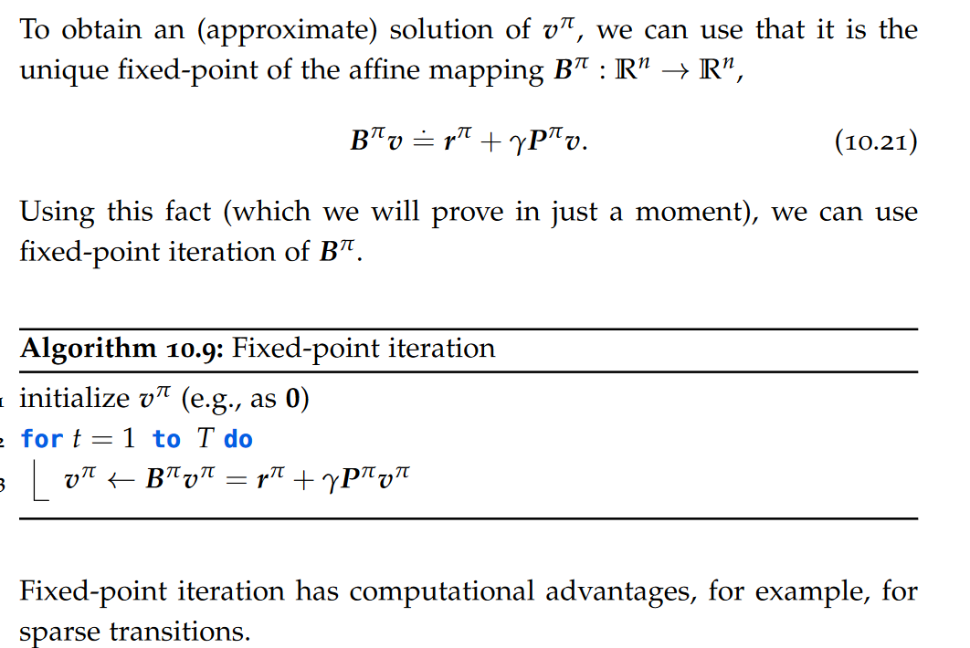
Policy Evaluation, Fixed-point Iteration, contraction,Banach fixed-point theorem

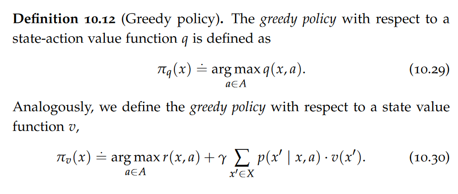
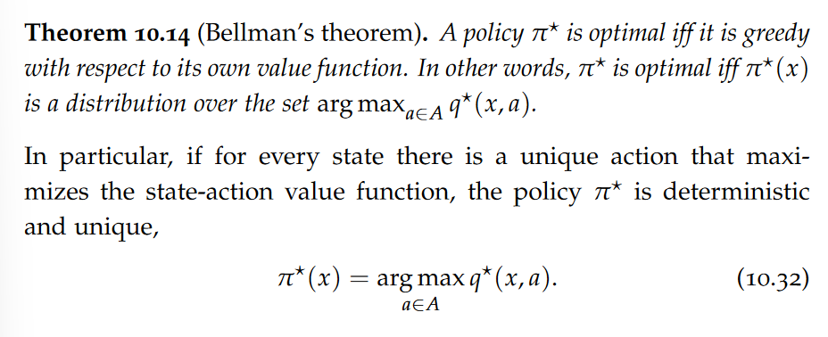
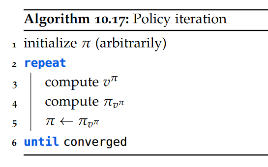
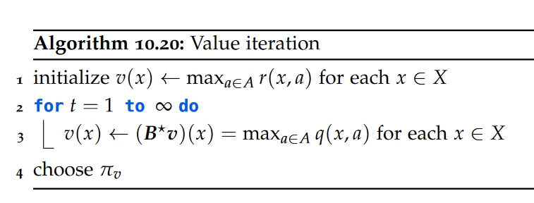
Policy Optimization, Greedy Policies, Bellman Optimality Equation, Bellman’s theorem, Policy Iteration, Value Iteration,

In particular, if for every state there is a unique action that maximizes the state-action value function, the policy π⋆ is deterministic and unique.

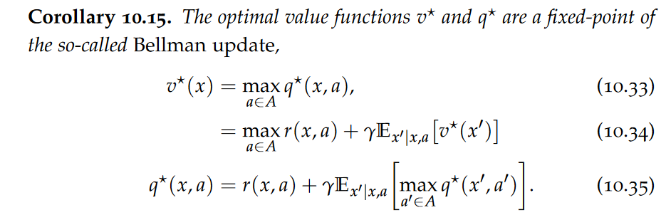
Intuitively, the Bellman optimality equations express that the value of a state under an optimal policy must equal the expected return for the best action from that state.

Value iteration converges to an ε-optimal solution in a polynomial number of iterations. Unlike policy iteration, value iteration does not converge to an exact solution in general.

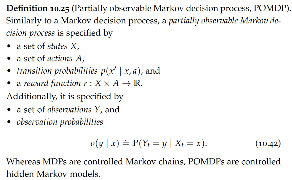
Partial Observability,

Whereas MDPs are controlled Markov chains, POMDPs are controlled hidden Markov models.

Tabular Reinforcement Learning

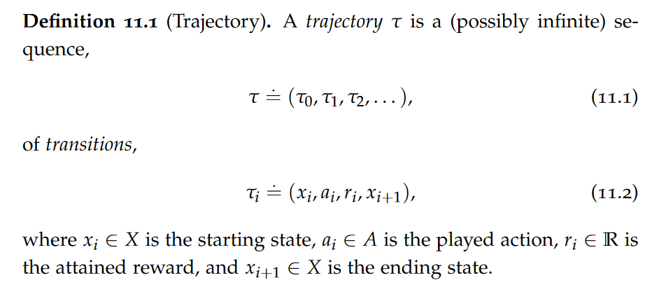
Trajectories, episodic setting, continuous setting, On-policy and Off-policy Methods,

on-policy methods are used when the agent has control over its own actions, in other words, the agent can freely choose to follow any policy. off-policy methods can be used even when the agent cannot freely choose its actions.

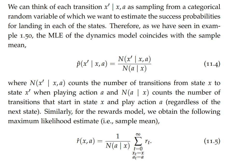
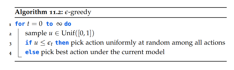
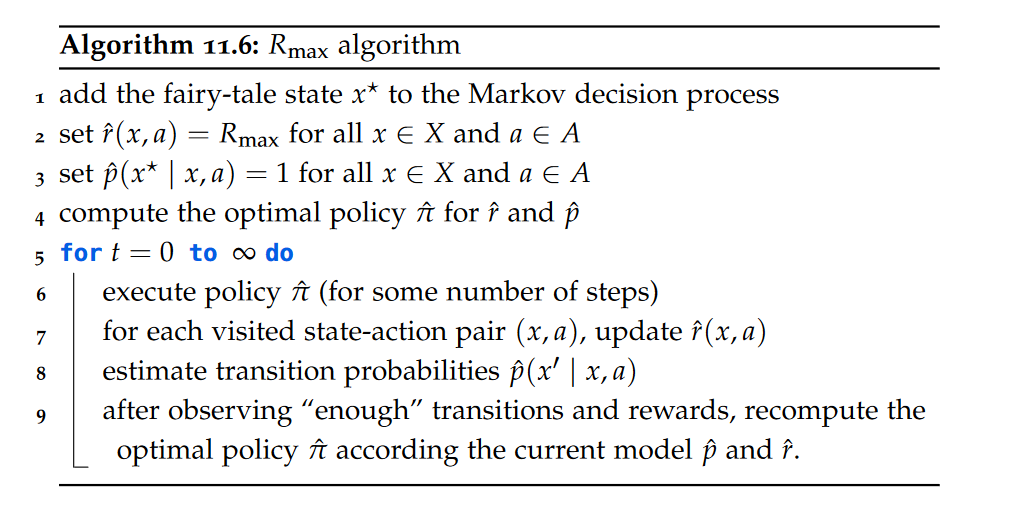
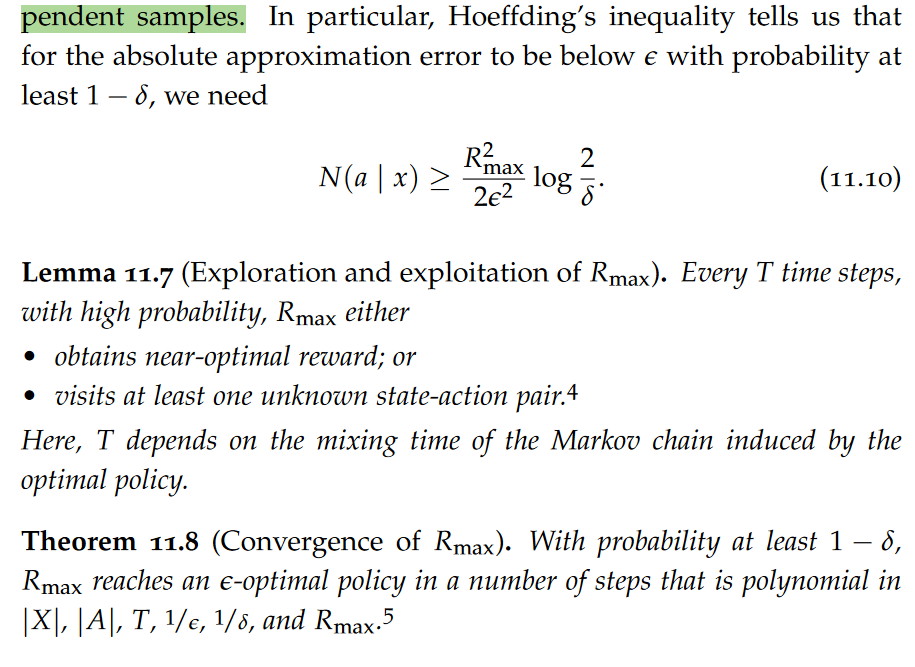
Model-based Approaches, Balancing Exploration and Exploitation, ε-greedy, Softmax Exploration(Boltzmann exploration), Rmax algorithm

skip Remark 11.3: Asymptotic convergence

Note that ε-greedy is GLIE with probability 1 if the sequence (εt)t∈N0 satisfies the RM-conditions (A.56), e.g., if εt = 1/t.

A significant benefit to model-based reinforcement learning is that it is inherently off-policy. That is, any trajectory regardless of the policy used to obtain it can be used to improve the model of the underlying Markov decision process. In the model-free setting, this not necessarily true.

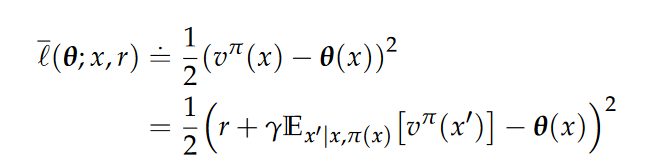
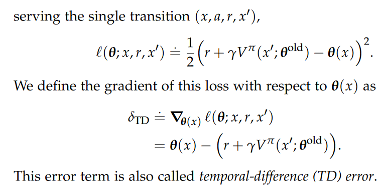
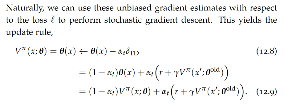
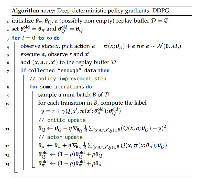
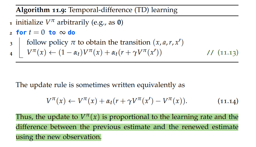
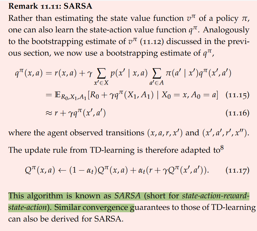
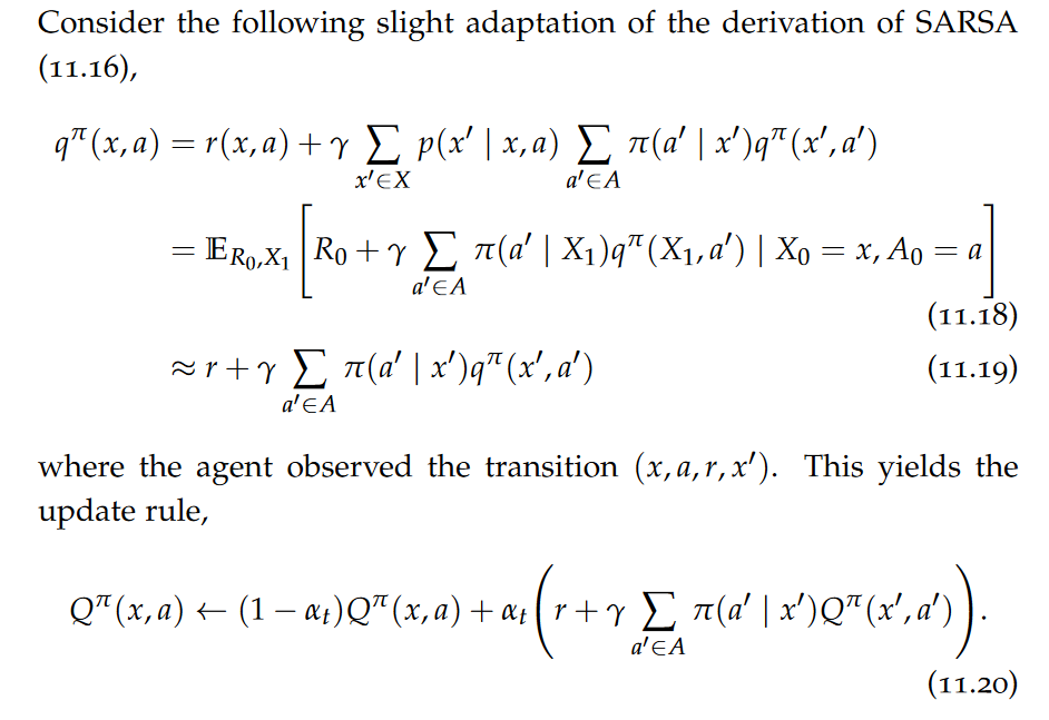
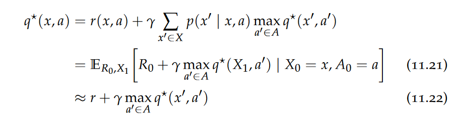
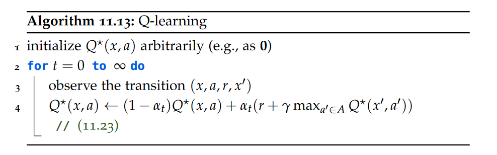
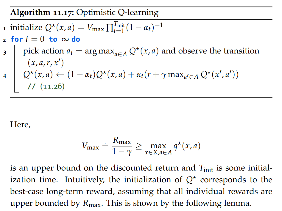
Model-free Approaches, On-policy Value Estimation, bootstrapping, temporal-difference learning, SARSA, Off-policy Value Estimation, Q-learning, optimistic Q-learning

Model-free Reinforcement Learning

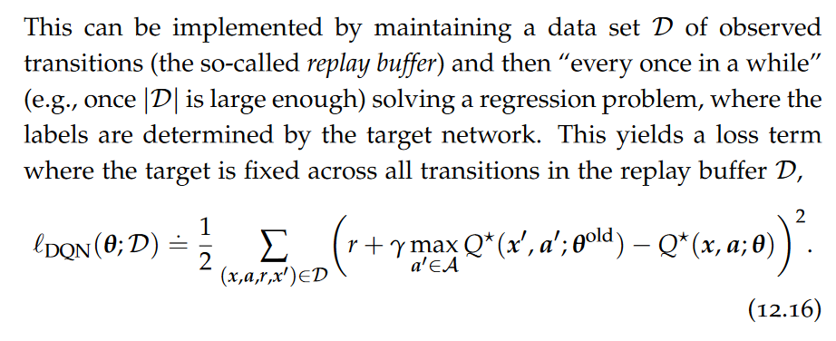
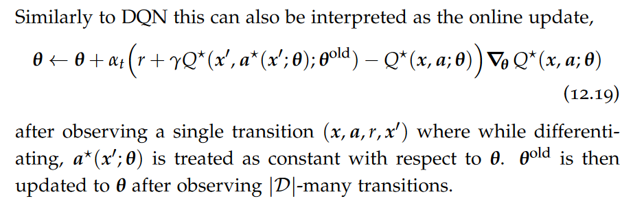
Value Function Approximation, DQN, experience replay, maximization bias, Double DQN

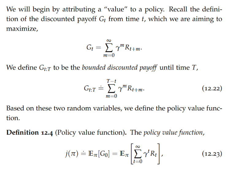
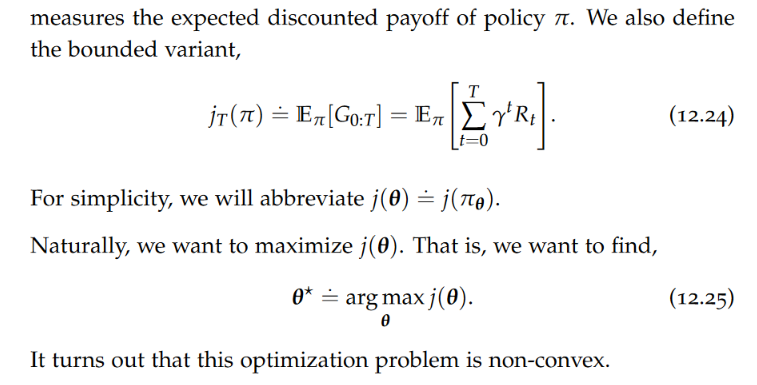
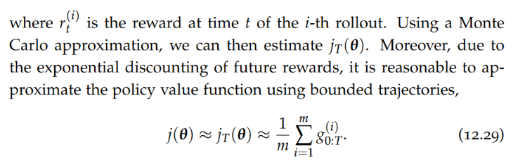
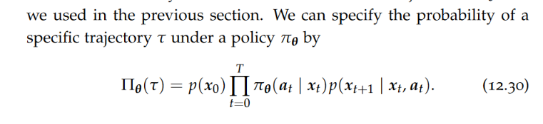
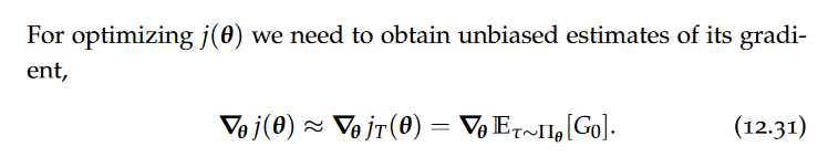
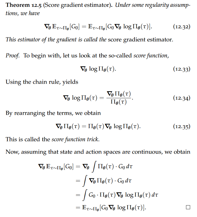
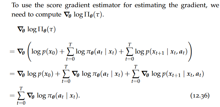
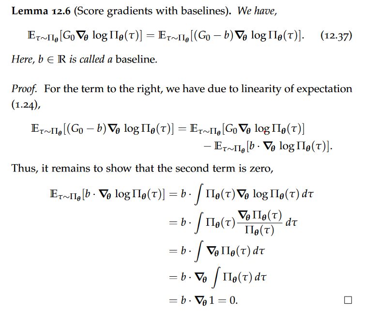
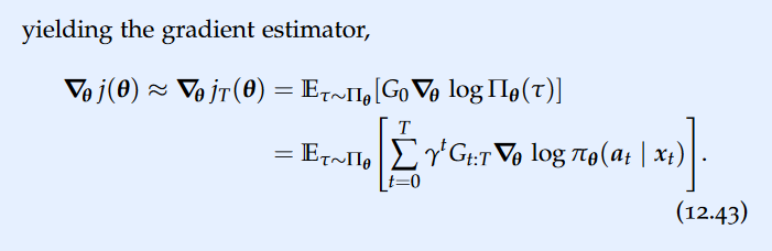
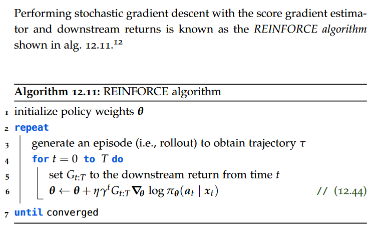
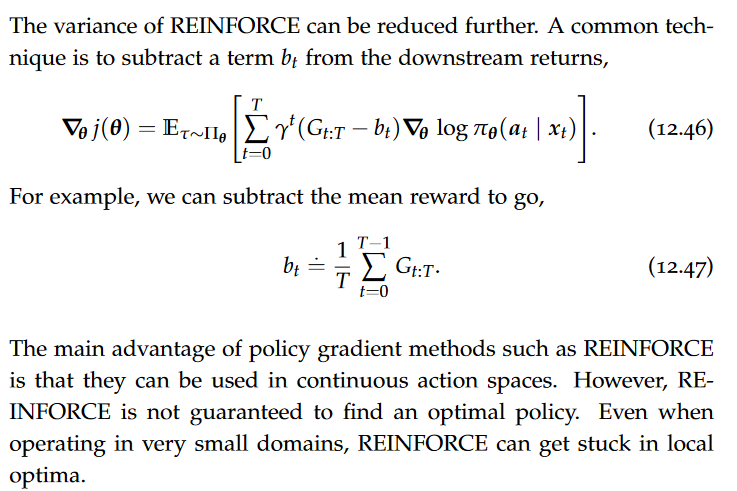
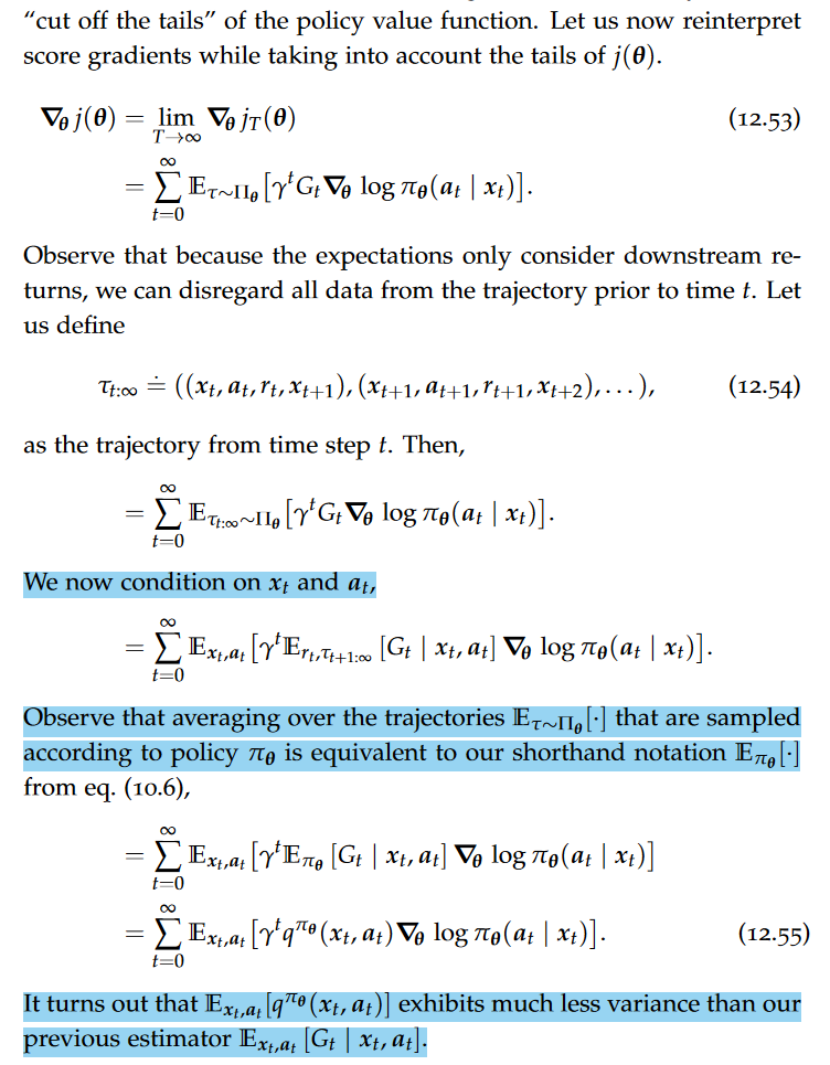
Policy Approximation(policy gradient methods), policy value function, Policy Gradient, Score gradient estimator, Score gradients with baselines, Downstream returns, REINFORCE algorithm

The main advantage of policy gradient methods such as REINFORCE is that they can be used in continuous action spaces. However, REINFORCE is not guaranteed to find an optimal policy. Even when operating in very small domains, REINFORCE can get stuck in local optima.

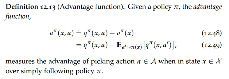
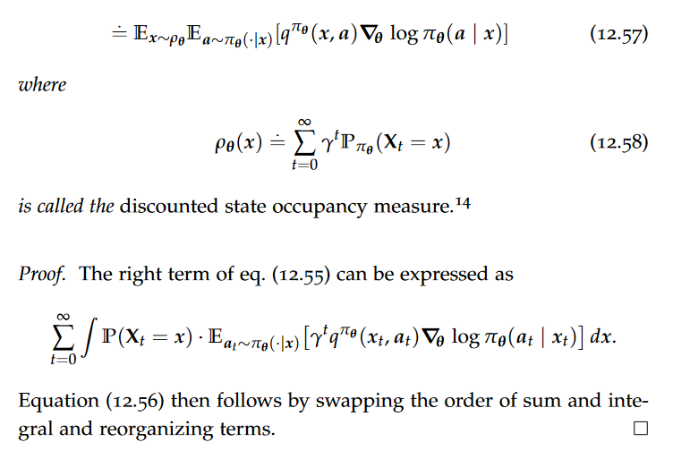
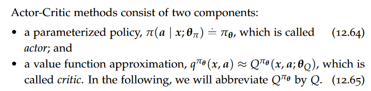
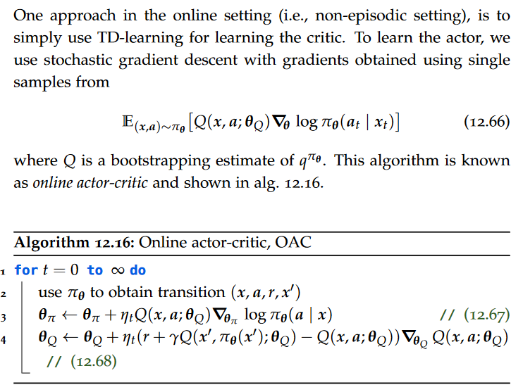
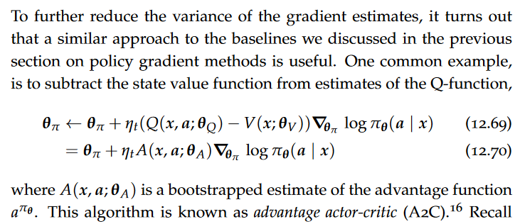
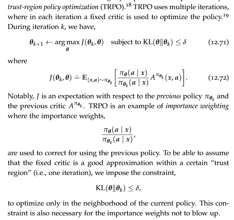
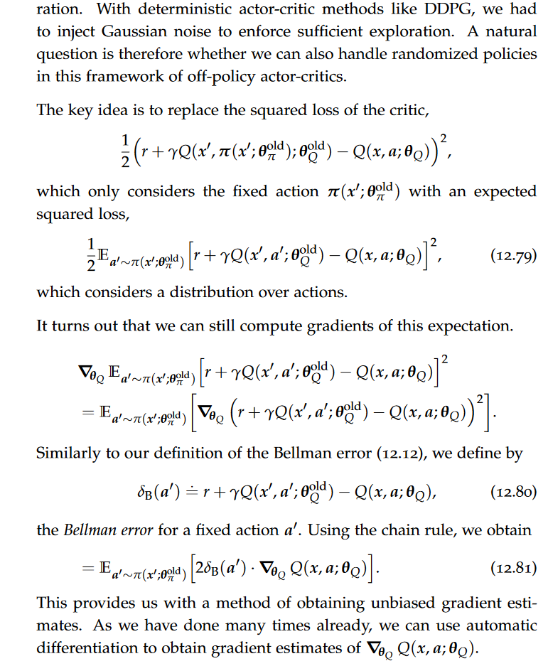
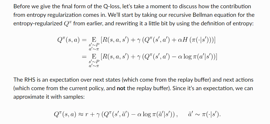
On-policy Actor-Critics,Advantage Function, Policy Gradient Theorem, Actor-Critic(Q actor-critic,Online actor-critic), advantage actor-critic, bias-variance tradeoff, trust-region policy optimization (TRPO), Proximal policy optimization (PPO)

One approach in the online setting (i.e., non-episodic setting), is to simply use SARSA for learning the critic. To learn the actor, we use stochastic gradient descent with gradients obtained using single samples.

Model-based Reinforcement Learning

Planning over Finite Horizons, receding horizon control (RHC), model predictive control (MPC), Random shooting methods

cheat sheet

from book

conditional distribution for gaussian;
Gaussian process posterior;
the predictive posterior at the test point;
common kernels;
the Hessian of the logistic loss;
Surprise,entropy,Jensen’s Inequality,Cross-entropy,KL-divergence,
ELBO,
the law of large numbers and Hoeffding’s inequality,
Hoeffding bound,

from exercise

Woodbury push-through identity;
Solution to problem 3.6;

model-based reinforcement learning

We face three main challenges in model-based reinforcement learning. First, given a fixed model, we need to perform planning to decide on which actions to play. Second, we need to learn models f and r accurately and efficiently. Third, we need to effectively trade exploration and exploitation.

Planning

Deterministic Dynamics

To begin with, let us assume that our dynamics model is deterministic and known. That is, given a state-action pair, we know the subsequent state.

Model-free Approximate Reinforcement Learning

Tabular Reinforcement Learning as Optimization

In particular, in the tabular setting (i.e., over a discrete domain), we can parameterize the value function exactly by learning a separate parameter for each state.

Now, we cannot compute this derivative because we cannot compute the expectation. Firstly, the expectation is over the true value function which is unknown to us. Secondly, the expectation is over the transition model which we are trying to avoid in model-free methods. To resolve the first issue, analogously to TD-learning, instead of learning the true value function vπ which is unknown, we learn the bootstrapping estimate Vπ. To resolve the first issue, analogously to TD-learning, instead of learning the true value function vπ which is unknown, we learn the bootstrapping estimate Vπ. we will use a Monte Carlo estimate using a single sample. Recall that this is only possible because the transitions are conditionally independent given the state-action pair.

Therefore, TD-learning is essentially performing stochastic gradient descent using the TD-error as an unbiased gradient estimate.
Stochastic gradient descent with a bootstrapping estimate is also called stochastic semi-gradient descent.

Value Function Approximation

Our goal for large state-action spaces is to exploit the smoothness properties5 of the value function to condense the representation.

Heuristics

The vanilla stochastic semi-gradient descent is very slow.
There are mainly two problems.
As we are trying to learn an approximate value function that depends on the bootstrapping estimate, this means that the optimization target is “moving” between iterations. In practice, moving targets lead to stability issues. One such technique aiming to “stabilize” the optimization targets is called neural fitted Q-iteration or deep Q-networks (DQN). DQN updates the neural network used for the approximate bootstrapping estimate infrequently to maintain a constant optimization target across multiple episodes. One approach is to clone the neural network and maintain one changing neural network (“online network”) for the most recent estimate of the Q-function which is parameterized by θ, and one fixed neural network (“target network”) used as the target which is parameterized by θold and which is updated infrequently.

This technique is known as experience replay. Another approach is Polyak averaging where the target network is gradually “nudged” by the neural network used to estimate the Q function.

Now, observe that the estimates Q⋆ are noisy estimates of q⋆. The fact that the update rules can be affected by inaccuracies (i.e., noise in the estimates) of the learned Q-function is known as the “maximization bias”. Double DQN (DDQN) is an algorithm that addresses this maximization bias. Instead of picking the optimal action with respect to the old network, it picks the optimal action with respect to the new network. Intuitively, this change ensures that the evaluation of the target network is consistent with the updated Q-function, which makes it more difficult for the algorithm to be affected by noise.

Policy Approximation

Methods that find an approximate policy are also called policy search methods or policy gradient methods. Policy gradient methods use randomized policies for encouraging exploration.

Estimating Policy Values

The policy value function measures the expected discounted payoff of policy π.

Reinforce Gradient

In this context, however, we cannot apply the reparameterization trick. Fortunately, there is another way of estimating this gradient.

When using a neural network for the parameterization of the policy π, we can use automatic differentiation to obtain unbiased gradient estimates. However, it turns out that the variance of these estimates is very large. Using so-called baselines can reduce the variance dramatically.

The baseline essentially captures the expected or average value, providing a reference point. By subtracting this reference point, the updates become more focused on the deviations from the expected values, which can reduce the variance in these deviations.

Typically, policy gradient methods are slow due to the large variance in the score gradient estimates. Because of this, they need to take small steps and require many rollouts of a Markov chain. Moreover, we cannot reuse data from previous rollouts, as policy gradient methods are fundamentally on-policy.

Actor-Critic Methods

Actor-Critic methods reduce the variance of policy gradient estimates by using ideas from value function approximation. They use function approximation both to approximate value functions and to approximate policies.

Advantage Function

Intuitively, the advantage function is a shifted version of the state-action function q that is relative to 0. It turns out that using this quantity instead, has numerical advantages.

Policy Gradient Theorem

Intuitively, ρθ(x) measures how often we visit state x when following policy πθ. It can be thought of as a “discounted frequency”. Importantly, ρθ is not a probability distribution, as it is not normalized to integrate to 1. Instead, ρθ is what is often called a finite measure. Therefore, eq. (12.57) is not a real expectation!

On-policy Actor-Critics

OAC

Due to the use of TD-learning for learning the critic, this algorithm is fundamentally on-policy.

A2C

that the Q-function is an absolute quantity, whereas the advantage function is a relative quantity, where the sign is informative for the gradient direction. Intuitively, an absolute value is harder to estimate than the sign. Actor-Critic methods are therefore often implemented with respect to the advantage function rather than the Q-function.

GAE/GAAE

Taking a step back, observe that the policy gradient methods such as REINFORCE generally have high variance in their gradient estimates. However, due to using Monte Carlo estimates of Gt, the gradient estimates are unbiased. In contrast, using a bootstrapped Q-function to obtain gradient estimates yields estimates with a smaller variance, but those estimates are biased. We are therefore faced with a bias-variance tradeoff. A natural approach is therefore to blend both gradient estimates to allow for effectively trading bias and variance. This leads to algorithms such as generalized advantage estimation (GAE/GAAE).

Improving sample efficiency(TRPO/PPO)

Actor-Critic methods generally suffer from low sample efficiency. One well-known variant that slightly improves the sample efficiency is trust-region policy optimization (TRPO).

Intuitively, taking the expectation with respect to the previous policy πθk , means that we can reuse data from rollouts within the same iteration. TRPO allows reusing past data as long as it can still be “trusted”. This makes TRPO “somewhat” off-policy. Fundamentally, though, TRPO is still an on-policy method. Proximal policy optimization (PPO) is a heuristic variant of TRPO that often works well in practice.

Off-policy Actor-Critics

These algorithms use the reparameterization gradient estimates, instead of score gradient estimators.

DDPG

As our method is off-policy, a simple idea in continuous action spaces is to add Gaussian noise to the action selected by πθ — also known as Gaussian noise “dithering”. This corresponds to an algorithm called deep deterministic policy gradients.
This algorithm is essentially equivalent to Q-learning with function approximation (e.g., DQN), with the only exception that we replace the maximization over actions with the learned policy πθ.

Twin delayed DDPG (TD3) is an extension of DDPG that uses two separate critic networks for predicting the maximum action and evaluating the policy. This addresses the maximization bias akin to Double-DQN. TD3 also applies delayed updates to the actor network, which increases stability.

Off-Policy Actor Critics with Randomized Policies

The algorithm that uses eq. (12.81) to obtain gradients for the critic and reparameterization gradients for the actor is called stochastic value gradients (SVG).

Off-policy Actor-Critics with Entropy Regularization

In practice, algorithms like SVG often do not explore enough. A key issue with relying on randomized policies for exploration is that they might collapse to deterministic policies.

A simple trick that encourages a little bit of extra exploration is to regularize the randomized policies “away” from putting all mass on a single action. This approach is known as entropy regularization and it leads to an analogue of Markov decision processes called entropy-regularized Markov decision process, where suitably defined regularized state-action value functions (so-called soft value functions) are used.

soft actor critic(SAC)

references

https://towardsdatascience.com/soft-actor-critic-demystified-b8427df61665
https://github.com/tsmatz/reinforcement-learning-tutorials/blob/master/06-sac.ipynb
https://spinningup.openai.com/en/latest/algorithms/sac.html
https://towardsdatascience.com/policy-gradients-in-a-nutshell-8b72f9743c5d
https://lilianweng.github.io/posts/2018-04-08-policy-gradient/

Tabular Reinforcement Learning

The Reinforcement Learning Problem

Reinforcement learning is concerned with probabilistic planning in unknown environments. In this chapter, we will begin by considering reinforcement learning with small state and action spaces. This setting is often called the tabular setting, as the value functions can be computed exhaustively for all states and stored in a table.

Clearly, the agent needs to trade exploring and learning about the environment with exploiting its knowledge to maximize rewards. In fact, Bayesian optimization can be viewed as reinforcement learning with a fixed state and a continuous action space: In each round, the agent plays an action, aiming to find the action that maximizes the reward.Another key challenge of reinforcement learning is that the observed data is dependent on the played actions.

Trajectories

Crucially, the newly observed states xt+1 and the rewards rt (across multiple transitions) are conditionally independent given the previous states xt and actions at. This independence property is crucial for being able to learn about the underlying Markov decision process. Notably, this implies that we can apply the law of large numbers (1.83) and Hoeffding’s inequality (1.87) to our estimators of both quantities.

The collection of data is commonly classified into two settings. In the episodic setting, the agent performs a sequence of “training” rounds (called episodes). In the beginning of each round, the agent is reset to some initial state. In contrast, in the continuous setting (or non-episodic,or online setting), the agent learns online.

control

Another important distinction in how data is collected, is the distinction between on-policy and off-policy control. As the names suggest, on-policy methods are used when the agent has control over its own actions, in other words, the agent can freely choose to follow any policy. In contrast, off-policy methods can be used even when the agent cannot freely choose its actions. Off-policy methods are therefore able to make use of observational data.Off-policy methods are therefore more sample-efficient than on-policy methods. This is crucial, especially in settings where conducting experiments (i.e., collecting new data) is expensive.

On-Policy learning algorithms are the algorithms that evaluate and improve the same policy which is being used to select actions. Off-Policy learning algorithms evaluate and improve a policy that is different from Policy that is used for action selection.

To understand the difference between on-policy learning and off-policy learning one must first understand the difference between the behavior policy (i.e., sampling policy) and the update policy. The behavior policy is the policy an agent follows when choosing which action to take in the environment at each time step. The update policy is how the agent updates the Q-function. On-policy algorithms attempt to improve upon the current behavior policy that is used to make decisions and therefore these algorithms learn the value of the policy carried out by the agent, Off-policy algorithms learn the value of the optimal policy and can improve upon a policy that is different from the behavior policy. Determining if the update and behavior policy are the same or different can give us insight into whether or not the algorithm is on-policy or off-policy.

Model-based Approaches

Approaches to reinforcement learning are largely categorized into two classes. Model-based approaches aim to learn the underlying Markov decision process. In contrast, model-free approaches learn the value function directly.

Learning the Underlying Markov Decision Process

A natural first idea is to use maximum likelihood estimation to approximate transition and reward function.

ε-greedy Algorithm

The key problem of ε-greedy is that it explores the state space in an uninformed manner. In other words, it explores ignoring all past experience. It thus does not eliminate clearly suboptimal actions.

Rmax Algorithm

A key principle in effectively trading exploration and exploitation is “optimism in the face of uncertainty”. Let us apply this principle to the reinforcement learning setting. The key idea is to assume that the dynamics and rewards model “work in our favor” until we have learned “good estimates” of the true dynamics and rewards.

How many transitions are “enough”? We can use Hoeffding’s inequality to get a rough idea!

challenges

Model-free Approaches

A significant benefit to model-based reinforcement learning is that it is inherently off-policy. That is, any trajectory regardless of the policy used to obtain it can be used to improve the model of the underlying Markov decision process. In the model-free setting, this not necessarily true.

On-policy Value Estimation

Note that to estimate this expectation we use a single(!) sample.However, there is one significant problem in this approximation. Our approximation of vπ does in turn depend on the (unknown) true value of vπ. The key idea is to use a bootstrapping estimate of the value function instead. That is, in place of the true value function vπ, we will use a “running estimate” Vπ. In other words, whenever observing a new transition, we use our previous best estimate of vπ to obtain a new estimate Vπ.

Crucially, using a bootstrapping estimate generally results in biased estimates of the value function. Moreover, due to relying on a single sample, the estimates tend to have very large variance.

TD-learning

The variance of the estimate is typically reduced by mixing new estimates of the value function with previous estimates using a learning rate αt. This yields the temporal-difference learning algorithm.

TD-learning is a fundamentally on-policy method. That is, for the estimates Vπ to converge to the true value function vπ, the transitions that are used for the estimation must follow policy π.

SARSA

Off-policy Value Estimation

This adapted update rule explicitly chooses the subsequent action a′ according to policy π whereas SARSA absorbs this choice into the Monte Carlo approximation. The algorithm has analogous convergence guarantees to those of SARSA. Crucially, this algorithm is off-policy. As noted, the key difference to the on-policy TD-learning and SARSA is that our estimate of the Qfunction explicitly keeps track of the next-performed action. It does so for any action in any state.

Q-learning

Crucially, the Monte Carlo approximation of eq. (11.21) does not depend on the policy. Thus, Q-learning is an off-policy method.

Optimistic Q-learning

Challenges

We have seen that both the model-based Rmax algorithm and the modelfree Q-learning take time polynomial in the number of states |X| and the number of actions |A| to converge. While this is acceptable in small grid worlds, this is completely unacceptable for large state and action spaces.

references

https://core-robotics.gatech.edu/2022/02/28/bootcamp-summer-2020-week-4-on-policy-vs-off-policy-reinforcement-learning/

Markov Decision Processes

Planning deals with the problem of deciding which action an agent should play in a (stochastic) environment(An environment is stochastic as opposed to deterministic, when the outcome of actions is random.). A key formalism for probabilistic plan ning in known environments are so-called Markov decision processes.

Our fundamental objective is to learn how the agent should behave to optimize its reward. In other words, given its current state, the agent should decide (optimally) on the action to play. Such a decision map — whether optimal or not — is called a policy.

For the purpose of our discussion of Markov decision processes and reinforcement learning, we will focus on a very common reward called discounted payoff.

Because we assumed stationary dynamics, rewards, and policies, the discounted payoff starting from a given state x will be independent of the start time t.

Bellman Expectation Equation

Let us now see how we can compute the value function：

This equation is known as the Bellman expectation equation, and it shows a recursive dependence of the value function on itself. The intuition is clear: the value of the current state corresponds to the reward from the next action plus the discounted sum of all future rewards obtained from the subsequent states.

Policy Evaluation

Bellman’s expectation equation tells us how we can find the value function vπ of a fixed policy π using a system of linear equations.

Fixed-point Iteration

Policy Optimization

Greedy Policies

Bellman Optimality Equation

These equations are also called the Bellman optimality equations. Intuitively, the Bellman optimality equations express that the value of a state under an optimal policy must equal the expected return for the best action from that state. Bellman’s theorem is also known as Bellman’s optimality principle, which is a more general concept.

Policy Iteration

It can be shown that policy iteration converges to an exact solution in a polynomial number of iterations.Each iteration of policy iteration requires computing the value function, which we have seen to be of cubic complexity in the number of states.

Value Iteration

Value iteration converges to an ε-optimal solution in a polynomial number of iterations. Unlike policy iteration, value iteration does not converge to an exact solution in general.an iteration of 7 Sparsity refers to the interconnectivity of the state space. When only few states are reachable from any state, we call an MDP sparse. value iteration can be performed in (virtually) constant time in sparse Markov decision processes.

Partial Observability

In this section, we consider how Markov decision processes can be extended to a partially observable setting where the agent can only access noisy observations Yt of its state Xt.

Observe that a Kalman filter can be viewed as a hidden Markov model with conditional linear Gaussian motion and sensor models and a Gaussian prior on the initial state.

POMDPs can be reduced to a Markov decision process with an enlarged state space.

Bayesian Optimization

Exploration-Exploitation Dilemma

In Bayesian optimization, we want to learn a model of f ⋆ and use this model to optimize f ⋆ simultaneously. These goals are somewhat contrary. Learning a model of f ⋆ requires us to explore the input space while using the model to optimize f ⋆ requires us to focus on the most promising well-explored areas. This trade-off is commonly known as the exploration-exploitation dilemma.

It is common to use a so-called acquisition function to greedily pick the next point to sample based on the current model.

Online Learning and Bandits

Multi-Armed Bandits(MAB)

The “multi-armed bandits” (MAB) problem is a classical, canonical formalization of the exploration-exploitation dilemma. In the MAB problem, we are provided with k possible actions (arms) and want to maximize our reward online within the time horizon T. We do not know the reward distributions of the actions in advance, however, so we need to trade learning the reward distribution with following the most promising action.

Bayesian optimization can be interpreted as a variant of the MAB problem where there can be a potentially infinite number of actions (arms), but their rewards are correlated (because of the smoothness of the Gaussian process prior). Smoothness means that nearby points in the input space are likely to have similar function values. Because of the smoothness property inherent in the Gaussian process prior, Bayesian optimization can make informed decisions about where to explore next in the input space. The model can leverage information from previously evaluated points to predict the behavior of the objective function at unexplored points more effectively.

Regret

The key performance metric in online learning is the regret.

Achieving sublinear regret requires balancing exploration with exploitation. Typically, online learning (and Bayesian optimization) consider stationary environments, hence the comparison to the static optimum.

Acquisition Functions

Throughout our description of acquisition functions, we will focus on a setting where we model $f^⋆$ using a Gaussian process which we denote by f. The methods generalize to other means of learning $f^⋆$ such as Bayesian neural networks.

One possible acquisition function is uncertainty sampling. However, this acquisition function does not at all take into account the objective of maximizing $f^⋆$ and focuses solely on exploration.

Suppose that our model f of $f^⋆$ is well-calibrated, in the sense that the true function lies within its confidence bounds. Consider the best lower bound, that is, the maximum of the lower confidence bound. Now, if the true function is really contained in the confidence bounds, it must hold that the optimum is somewhere above this best lower bound.

Therefore, we only really care how the function looks like in the regions where the upper confidence bound is larger than the best lower bound. The key idea behind the methods that we will explore is to focus exploration on these plausible maximizers.

Upper Confidence Bound

This acquisition function naturally trades exploitation by preferring a large posterior mean with exploration by preferring a large posterior variance.
This optimization problem is non-convex in general. However, we can use approximate global optimization techniques like Lipschitz optimization (in low dimensions) and gradient ascent with random initialization (in high dimensions). Another widely used option is to sample some random points from the domain, score them according to this criterion, and simply take the best one.

Observe that if the information gain is sublinear in T then we achieve sublinear regret and, in particular, converge to the true optimum. The term “sublinear” refers to a growth rate that is slower than linear.

Intuitively, to work even if the unknown function $f^⋆$ is not contained in the confidence bounds, we use βt to re-scale the confidence bounds to enclose $f^⋆$.

Probability of Improvement

Probability of improvement tends to be biased in favor of exploitation, as it prefers points with large posterior mean and small posterior variance.

Expected Improvement

Intuitively, expected improvement seeks a large expected improvement (exploitation) while also preferring states with a large variance (exploration).

Thompson Sampling

Probability matching is exploratory as it prefers points with larger variance (as they automatically have a larger chance of being optimal), but at the same time exploitative as it effectively discards points with low posterior mean and low posterior variance. Unfortunately, it is generally difficult to compute π analytically given a posterior. Instead, it is common to use a sampling-based approximation of π.

In many cases, the randomness in the realizations of ̃ ft+1 is already sufficient to effectively trade exploration and exploitation.

Model Selection

Selecting a model of f ⋆ is much harder than in the i.i.d. data setting of supervised learning. There are mainly the two following dangers, • the data sets collected in active learning and Bayesian optimization are small; and • the data points are selected dependently on prior observations. This leads to a specific danger of overfitting. In particular, due to feedback loops between the model and the acquisition function, one may end up sampling the same point repeatedly.

Another approach that often works fairly well is to occasionally (according to some schedule) select points uniformly at random instead of using the acquisition function. This tends to prevent getting stuck in suboptimal parts of the state space.

difference betwwen active learning and Bayesian Optimization

Problem Setting:
Active Learning: Active learning typically deals with supervised learning tasks where there is a large pool of unlabeled instances, and the algorithm decides which instances to query for labels to improve the model.
Bayesian Optimization: Bayesian optimization deals with optimization problems where the objective function is unknown, expensive to evaluate, and possibly noisy. It aims to find the global optimum with as few evaluations as possible.

Nature of Queries:
Active Learning: In active learning, the queries are often in the form of “Which instance should be labeled next?” The goal is to select instances that will most benefit the model’s learning process.
Bayesian Optimization: In Bayesian optimization, the queries are in the form of “What point should be evaluated next in the input space to maximize/minimize the objective function?” The goal is to efficiently explore the input space and find the optimal configuration.

Algorithmic Approaches:
Active Learning: Active learning involves various strategies such as uncertainty sampling, query-by-committee, and diversity sampling to select informative instances for labeling.
Bayesian Optimization: Bayesian optimization employs probabilistic surrogate models (often Gaussian processes) to model the unknown objective function. Acquisition functions guide the search to balance exploration and exploitation efficiently.

Active learning

Active learning is a machine learning paradigm in which a model is trained on a dataset that is not entirely labeled. Instead of relying solely on a fully labeled dataset for training, active learning involves an iterative process where the model actively selects the most informative instances from an unlabeled pool, queries an oracle (typically a human annotator), and adds the newly labeled instances to the training set. The model is then retrained on the expanded labeled dataset.

The key idea behind active learning is to strategically choose the most valuable instances for labeling, with the goal of improving the model’s performance while minimizing the number of labeled instances needed. This process is especially beneficial when obtaining labeled data is expensive or time-consuming.

Active learning strategies vary in how they select instances for labeling. Common strategies include uncertainty sampling (select instances where the model is uncertain), query-by-committee (select instances where different model hypotheses disagree), and diversity sampling (select instances to ensure diverse coverage of the input space).

Conditional Entropy

Intuitively, the conditional entropy of X given Y describes our average surprise about realizations of X given a particular realization of Y, averaged over all such possible realizations of Y. In other words, conditional entropy corresponds to the expected remaining uncertainty in X after we observe Y.

That is, the joint entropy of X and Y is given by the uncertainty about X and the additional uncertainty about Y given X.

Mutual Information

In words, we subtract the uncertainty left about X after observing Y from our initial uncertainty about X. This measures the reduction in our uncertainty in X (as measured by entropy) upon observing Y.

Thus, the mutual information between X and Y can be understood as the approximation error (or information loss) when assuming that X and Y are independent.

Thus, the conditional mutual information corresponds to the reduction of uncertainty in X when observing Y, given we already observed Z.

Following our introduction of mutual information, it is natural to answer the question “where should I collect data?” by saying “wherever mutual information is maximized”.

Submodularity of Mutual Information

That is, “adding” x to the smaller set A yields more marginal gain than adding x to the larger set B. In other words, the function F has “diminishing returns”. In this way, submodularity can be interpreted as a notion of “concavity” for discrete functions.

Maximizing Mutual Information

Uncertainty Sampling

Therefore, if f is modeled by a Gaussian and we assume homoscedastic noise, greedily maximizing mutual information corresponds to simply picking the point x with the largest variance. This strategy is also called uncertainty sampling.

Heteroscedastic Noise

Uncertainty sampling is clearly problematic if the noise is heteroscedastic. If there are a particular set of inputs with a large aleatoric uncertainty dominating the epistemic uncertainty, uncertainty sampling will continuously choose those points even though the epistemic uncertainty will not be reduced substantially.

Thus, we choose locations that trade large epistemic uncertainty with large aleatoric uncertainty. Ideally, we find a location where the epistemic uncertainty is large, and the aleatoric uncertainty is low, which promises a significant reduction of uncertainty around this location.

Classification

Here, uncertainty sampling corresponds to selecting samples that maximize the entropy of the predicted label yx.

SWAG(Stochastic Weight Averaging Gaussian)

This paper proposes a different approach to Bayesian deep learning: they use the information contained in the SGD trajectory to efficiently approximate the posterior distribution over the weights of the neural network [1].

SWA

This paper shows that simple averaging of multiple points along the trajectory of SGD, with a cyclical or constant learning rate, leads to better generalization than conventional training [2].

cyclical learning rate schedule

Calibration of Modern Neural Networks

Confidence calibration – the problem of predicting probability estimates representative of the true correctness likelihood – is important for classification models in many applications. Through extensive experiments, we observe that depth, width, weight decay, and Batch Normalization are important factors influencing calibration.

references

[1] Maddox W J, Izmailov P, Garipov T, et al. A simple baseline for bayesian uncertainty in deep learning[J]. Advances in neural information processing systems, 2019, 32.
[2] Izmailov P, Podoprikhin D, Garipov T, et al. Averaging weights leads to wider optima and better generalization[J]. arXiv preprint arXiv:1803.05407, 2018.
[3] Guo C, Pleiss G, Sun Y, et al. On calibration of modern neural networks[C]//International conference on machine learning. PMLR, 2017: 1321-1330.

Markov Chain Monte Carlo Methods

The key idea of Markov chain Monte Carlo methods is to construct a Markov chain, which is efficient to simulate and has the stationary distribution p.

Markov Chains

Intuitively, the Markov property states that future behavior is independent of past states given the present state.

Markov chains can be classified into different types based on their behavior. These classifications include time-homogeneous and time-inhomogeneous Markov chains, irreducible Markov chains, and periodic and aperiodic Markov chains.

We restrict our attention to time-homogeneous Markov chains. That is, the transition probabilities do not change over time, which can be characterized by a transition function.

Irreducible Markov chains are those in which every state can be reached from any other state, while periodic Markov chains exhibit a repeating pattern in their states. On the other hand, aperiodic Markov chains do not exhibit any regular pattern in their states. If there is no fixed period at which the probabilities return to the starting values, the chain is classified as aperiodic. Aperiodic Markov chains often display a more complex and unpredictable behavior compared to periodic ones.

Stationarity

Convergence

A Markov Chain is called ergodic, if there exists a finite t such that every state can be reached from every state in exactly t steps.

Fundamental theorem of ergodic Markov chains

Detailed Balance Equation

Ergodic Theorem

This result is the fundamental reason for why Markov chain Monte Carlo methods are possible. In practice, one observes that Markov chain Monte Carlo methods have a so-called “burn-in” time during which the distribution of the Markov chain does not yet approximate the posterior distribution well. Typically, the first t0 samples are therefore discarded. It is not clear in general how T and t0 should be chosen such that the estimator is unbiased, rather they have to be tuned.

Elementary Sampling Methods

Metropolis-Hastings Algorithm

Gibbs Sampling

A popular example of a Metropolis-Hastings algorithm is Gibbs sampling.

Intuitively, by re-sampling single coordinates according to the posterior distribution given the other coordinates, Gibbs sampling finds states that are successively “more” likely.

Langevin Dynamics

Gibbs Distributions

references

https://www.collimator.ai/reference-guides/what-is-a-aperiodic-markov-chain

Variational Inference

The fundamental idea behind variational inference is to approximate the true posterior distribution using a “simpler” posterior that is as close as possible to the true posterior.

$$p(\theta\mid x_{1:n},y_{1:n})=\frac1Zp(\theta,y_{1:n}\mid x_{1:n})\approx q(\theta\mid\lambda)\doteq q_{\lambda}(\theta)$$

where λ represents the parameters of the variational posterior q, also called variational parameters.

Laplace Approximation

A natural idea for approximating the posterior distribution is to use a Gaussian approximation (that is, a second-order Taylor approximation) around the mode of the posterior. Such an approximation is known as a Laplace approximation.

As an example, we will look at Laplace approximation in the context of Bayesian logistic regression. Bayesian logistic regression corresponds to Bayesian linear regression with a Bernoulli likelihood.

Intuitively, the Laplace approximation matches the shape of the true posterior around its mode but may not represent it accurately elsewhere — often leading to extremely overconfident predictions.

Inference with a Variational

$$\begin{aligned} p(y^{\star}\mid x^{\star},x_{1:n},y_{1:n})& =\int p(y^\star\mid x^\star,\boldsymbol{\theta})p(\boldsymbol{\theta}\mid x_{1:n},y_{1:n})d\boldsymbol{\theta} \\ &\approx\int p(y^\star\mid x^\star,\boldsymbol{\theta})q_\lambda(\boldsymbol{\theta})d\boldsymbol{\theta} &=\int\int p(y^\star\mid f^\star)p(f^\star\mid x^\star,\theta)q_\lambda(\theta)d\theta df^\star\\&=\int p(y^\star\mid f^\star)\int p(f^\star\mid x^\star,\theta)q_\lambda(\theta)d\theta df^\star\\&=\int p(y^\star\mid f^\star)q_\lambda(f^\star\mid x^\star)df^\star.\quad\quad \end{aligned}$$

Information Theory

Surprise

The surprise about an event with probability u is defined as $S[u] = -log u$.

Entropy

The entropy of a distribution p is the average surprise about samples from p.if the entropy of p is large, we are more uncertain about x ∼ p than if the entropy of p were low.

$$\mathbb{H}[p]\doteq\mathbb{E}_{x\sim p}[\mathbb{S}[p(x)]]=\mathbb{E}_{x\sim p}[-\log p(x)].$$

Cross-Entropy

Cross-entropy can also be expressed in terms of the KL-divergence. Quite intuitively, the average surprise in samples from p with respect to the distribution q is given by the inherent uncertainty in p and the additional surprise that is due to us assuming the wrong data distribution q. The “closer” q is to the true data distribution p, the smaller is the additional average surprise.

$$\mathrm{H}[p\|q]=\mathrm{H}[p]+\mathrm{KL}(p\|q)\geq\mathrm{H}[p].$$

Variational Families

We can view variational inference more generally as a family of approaches aiming to approximate the true posterior distribution by one that is closest (according to some criterion) among a “simpler” class of distributions.

Kullback-Leibler Divergence

In words, KL(p∥q) measures the additional expected surprise when observing samples from p that is due to assuming the (wrong) distribution q and which not inherent in the distribution p already. Intuitively, the KL-divergence measures the information loss when approximating p with q.

Forward and reverse KL-divergence

KL(p∥q) is also called the forward (or inclusive) KL-divergence. In contrast, KL(q∥p) is called the reverse (or exclusive) KL-divergence.

It can be seen that the reverse KL-divergence tends to greedily select the mode and underestimating the variance which, in this case, leads to an overconfident prediction. The forward KL-divergence, in contrast, is more conservative and yields what one could consider the “desired” approximation.

The reverse KL-divergence is typically used in practice. This is for computational reasons. In principle, if the variational family Q is “rich enough”, minimizing the forward and reverse KL-divergences will yield the same result.

There is a nice interpretation of minimizing the forward KullbackLeibler divergence of the approximation $q_\lambda$ with respect to the true distribution p as being equivalent to maximizing the marginal model likelihood on a sample of infinite size. This interpretation is not useful in the setting where p is a posterior distribution over model parameters θ as a maximum likelihood estimate requires samples from p which we cannot obtain in this case.

KL-divergence of Gaussians

Evidence Lower Bound

The Evidence Lower Bound is a quantity maximization of which is equivalent to minimizing the KL-divergence. As its name suggests, the evidence lower bound is a (uniform) lower bound to the log-evidence $log p(y{1:n}|x{1:n})$.

Note that this inequality lower bounds the logarithm of an integral by an expectation of a logarithm over some variational distribution q. Hence, the ELBO is a family of lower bounds — one for each variational distribution. Such inequalities are called variational inequalities.

Gradient of Evidence Lower Bound

Obtaining the gradient of the evidence lower bound is more difficult. This is because the expectation integrates over the measure $q_\lambda$, which depends on the variational parameters $\lambda$. Thus, we cannot move the gradient operator inside the expectation.

There are two main techniques which are used to rewrite the gradient in such a way that Monte Carlo sampling becomes possible. The first is to use score gradients. The second is the so-called reparameterization trick.

reparameterization trick

The procedure of approximating the true posterior using a variational posterior by maximizing the evidence lower bound using stochastic optimization is also called black box stochastic variational inference. The only requirement is that we can obtain unbiased gradient estimates from the evidence lower bound (and the likelihood).