pai - Markov Decision Processes

Markov Decision Processes

Planning deals with the problem of deciding which action an agent should play in a (stochastic) environment(An environment is stochastic as opposed to deterministic, when the outcome of actions is random.). A key formalism for probabilistic plan ning in known environments are so-called Markov decision processes.
Alt text

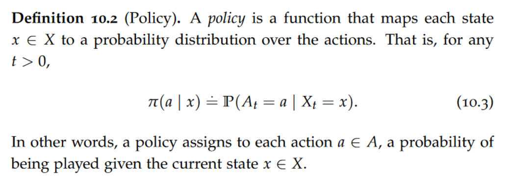
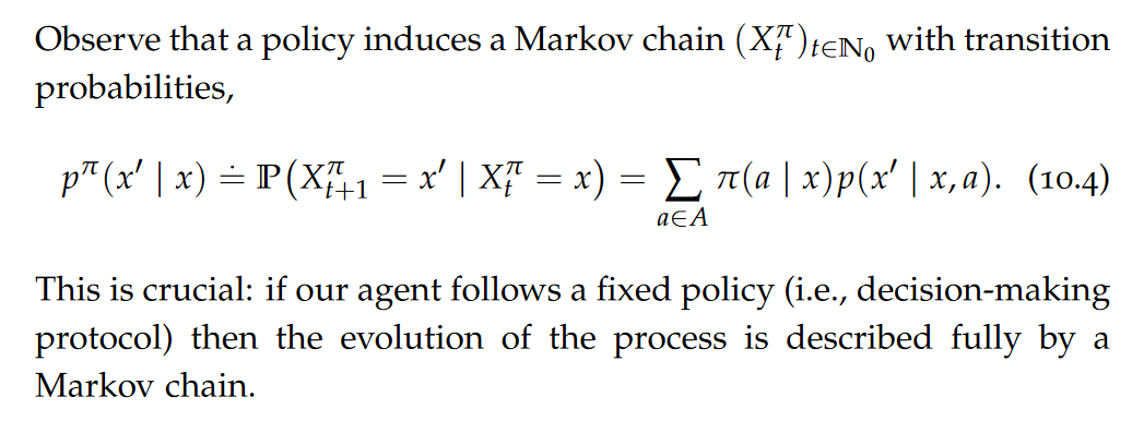
Our fundamental objective is to learn how the agent should behave to optimize its reward. In other words, given its current state, the agent should decide (optimally) on the action to play. Such a decision map — whether optimal or not — is called a policy.

Alt text

Alt text

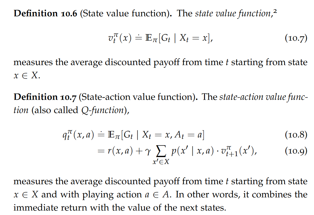
For the purpose of our discussion of Markov decision processes and reinforcement learning, we will focus on a very common reward called discounted payoff.

Alt text

Alt text

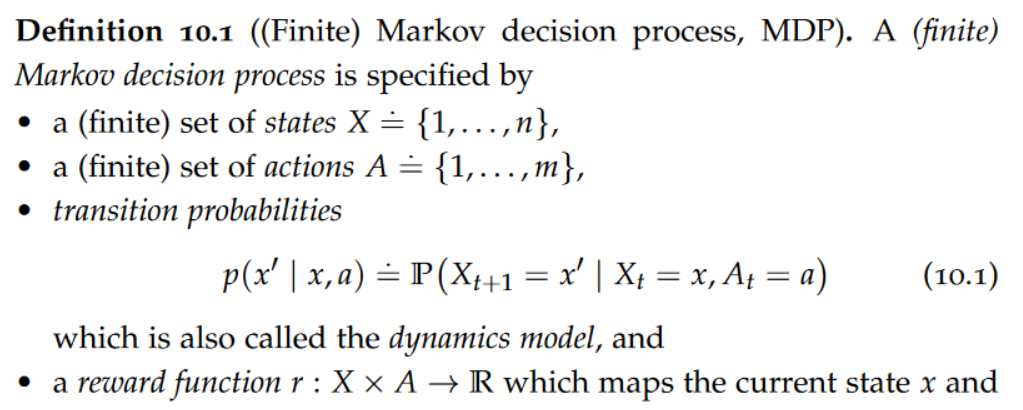
Because we assumed stationary dynamics, rewards, and policies, the discounted payoff starting from a given state x will be independent of the start time t.

Bellman Expectation Equation

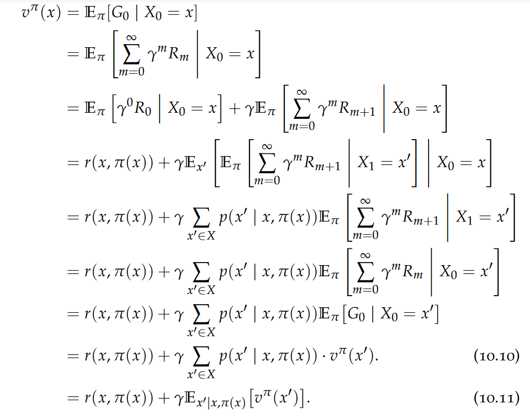
Let us now see how we can compute the value function:

Alt text

This equation is known as the Bellman expectation equation, and it shows a recursive dependence of the value function on itself. The intuition is clear: the value of the current state corresponds to the reward from the next action plus the discounted sum of all future rewards obtained from the subsequent states.

Policy Evaluation

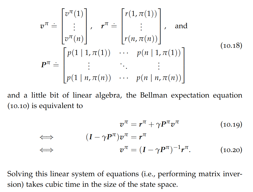
Bellman’s expectation equation tells us how we can find the value function vπ of a fixed policy π using a system of linear equations.

Alt text

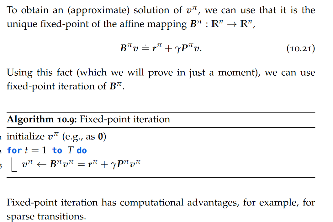
Fixed-point Iteration

Alt text

Policy Optimization

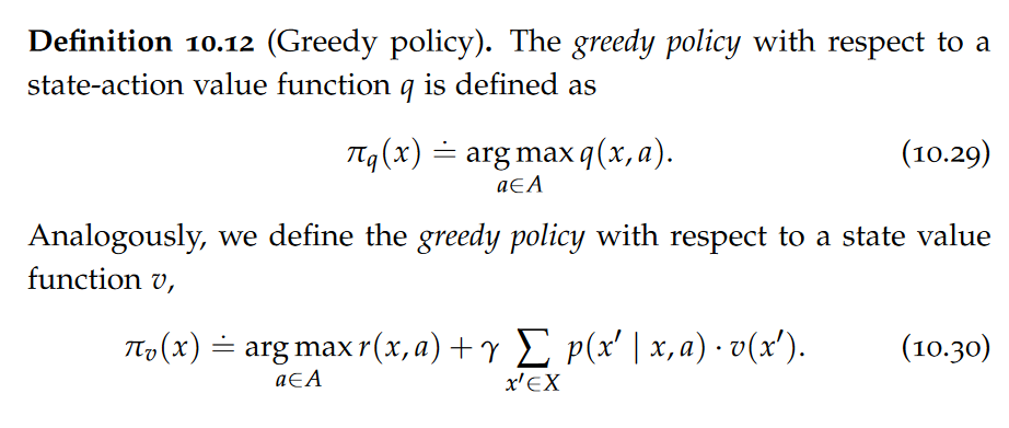
Greedy Policies

Alt text

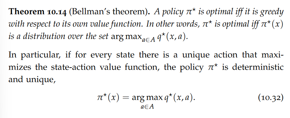
Bellman Optimality Equation

Alt text

Alt text
These equations are also called the Bellman optimality equations. Intuitively, the Bellman optimality equations express that the value of a state under an optimal policy must equal the expected return for the best action from that state. Bellman’s theorem is also known as Bellman’s optimality principle, which is a more general concept.

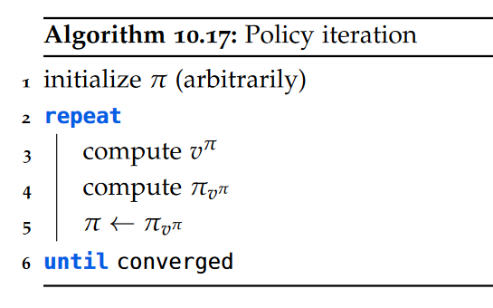
Policy Iteration

Alt text

It can be shown that policy iteration converges to an exact solution in a polynomial number of iterations.Each iteration of policy iteration requires computing the value function, which we have seen to be of cubic complexity in the number of states.

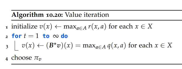
Value Iteration

Alt text
Value iteration converges to an ε-optimal solution in a polynomial number of iterations. Unlike policy iteration, value iteration does not converge to an exact solution in general.an iteration of 7 Sparsity refers to the interconnectivity of the state space. When only few states are reachable from any state, we call an MDP sparse. value iteration can be performed in (virtually) constant time in sparse Markov decision processes.

Partial Observability

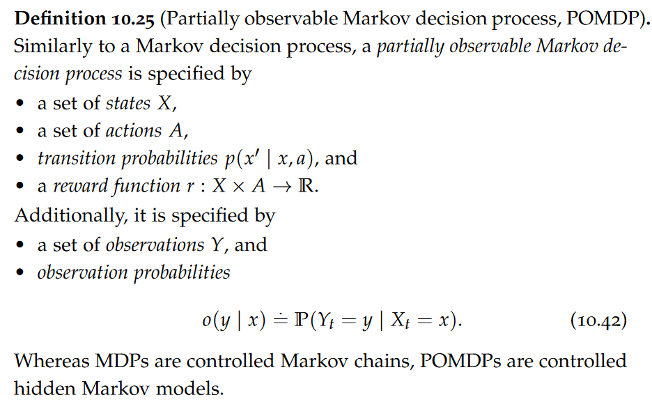
In this section, we consider how Markov decision processes can be extended to a partially observable setting where the agent can only access noisy observations Yt of its state Xt.

Alt text

Observe that a Kalman filter can be viewed as a hidden Markov model with conditional linear Gaussian motion and sensor models and a Gaussian prior on the initial state.

POMDPs can be reduced to a Markov decision process with an enlarged state space.

pai - Bayesian Optimization

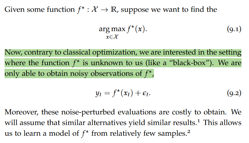
Bayesian Optimization

Alt text

Exploration-Exploitation Dilemma

In Bayesian optimization, we want to learn a model of f ⋆ and use this model to optimize f ⋆ simultaneously. These goals are somewhat contrary. Learning a model of f ⋆ requires us to explore the input space while using the model to optimize f ⋆ requires us to focus on the most promising well-explored areas. This trade-off is commonly known as the exploration-exploitation dilemma.

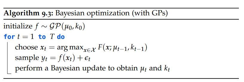
It is common to use a so-called acquisition function to greedily pick the next point to sample based on the current model.

Online Learning and Bandits

Alt text

Multi-Armed Bandits(MAB)

The “multi-armed bandits” (MAB) problem is a classical, canonical formalization of the exploration-exploitation dilemma. In the MAB problem, we are provided with k possible actions (arms) and want to maximize our reward online within the time horizon T. We do not know the reward distributions of the actions in advance, however, so we need to trade learning the reward distribution with following the most promising action.

Bayesian optimization can be interpreted as a variant of the MAB problem where there can be a potentially infinite number of actions (arms), but their rewards are correlated (because of the smoothness of the Gaussian process prior). Smoothness means that nearby points in the input space are likely to have similar function values. Because of the smoothness property inherent in the Gaussian process prior, Bayesian optimization can make informed decisions about where to explore next in the input space. The model can leverage information from previously evaluated points to predict the behavior of the objective function at unexplored points more effectively.

Regret

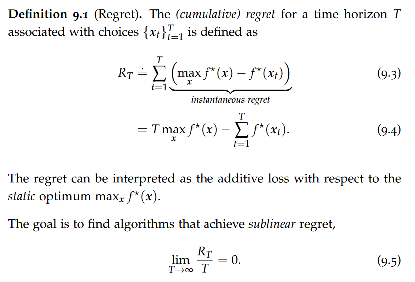
The key performance metric in online learning is the regret.

Alt text

Achieving sublinear regret requires balancing exploration with exploitation. Typically, online learning (and Bayesian optimization) consider stationary environments, hence the comparison to the static optimum.

Acquisition Functions

Throughout our description of acquisition functions, we will focus on a setting where we model $f^⋆$ using a Gaussian process which we denote by f. The methods generalize to other means of learning $f^⋆$ such as Bayesian neural networks.

Alt text

One possible acquisition function is uncertainty sampling. However, this acquisition function does not at all take into account the objective of maximizing $f^⋆$ and focuses solely on exploration.

Suppose that our model f of $f^⋆$ is well-calibrated, in the sense that the true function lies within its confidence bounds. Consider the best lower bound, that is, the maximum of the lower confidence bound. Now, if the true function is really contained in the confidence bounds, it must hold that the optimum is somewhere above this best lower bound.

Therefore, we only really care how the function looks like in the regions where the upper confidence bound is larger than the best lower bound. The key idea behind the methods that we will explore is to focus exploration on these plausible maximizers.

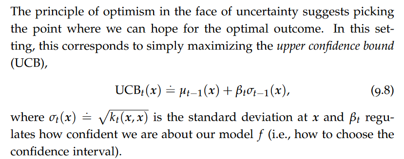
Upper Confidence Bound

Alt text
This acquisition function naturally trades exploitation by preferring a large posterior mean with exploration by preferring a large posterior variance.
This optimization problem is non-convex in general. However, we can use approximate global optimization techniques like Lipschitz optimization (in low dimensions) and gradient ascent with random initialization (in high dimensions). Another widely used option is to sample some random points from the domain, score them according to this criterion, and simply take the best one.

Alt text
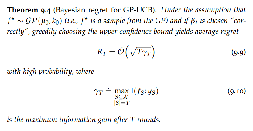
Observe that if the information gain is sublinear in T then we achieve sublinear regret and, in particular, converge to the true optimum. The term “sublinear” refers to a growth rate that is slower than linear.

Alt text
Intuitively, to work even if the unknown function $f^⋆$ is not contained in the confidence bounds, we use βt to re-scale the confidence bounds to enclose $f^⋆$.

Probability of Improvement

Alt text

Probability of improvement tends to be biased in favor of exploitation, as it prefers points with large posterior mean and small posterior variance.

Expected Improvement

Alt text

Intuitively, expected improvement seeks a large expected improvement (exploitation) while also preferring states with a large variance (exploration).

Thompson Sampling

Alt text

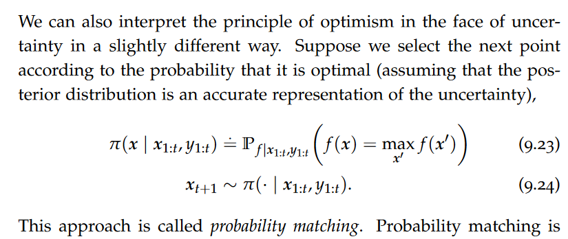
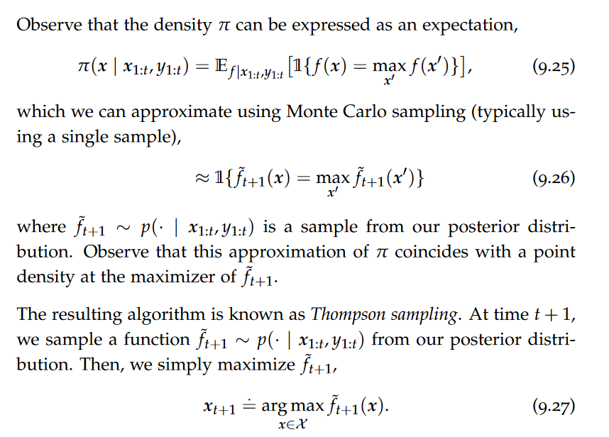
Probability matching is exploratory as it prefers points with larger variance (as they automatically have a larger chance of being optimal), but at the same time exploitative as it effectively discards points with low posterior mean and low posterior variance. Unfortunately, it is generally difficult to compute π analytically given a posterior. Instead, it is common to use a sampling-based approximation of π.

Alt text

In many cases, the randomness in the realizations of ̃ ft+1 is already sufficient to effectively trade exploration and exploitation.

Model Selection

Selecting a model of f ⋆ is much harder than in the i.i.d. data setting of supervised learning. There are mainly the two following dangers, • the data sets collected in active learning and Bayesian optimization are small; and • the data points are selected dependently on prior observations. This leads to a specific danger of overfitting. In particular, due to feedback loops between the model and the acquisition function, one may end up sampling the same point repeatedly.

Another approach that often works fairly well is to occasionally (according to some schedule) select points uniformly at random instead of using the acquisition function. This tends to prevent getting stuck in suboptimal parts of the state space.

difference betwwen active learning and Bayesian Optimization

Problem Setting:
Active Learning: Active learning typically deals with supervised learning tasks where there is a large pool of unlabeled instances, and the algorithm decides which instances to query for labels to improve the model.
Bayesian Optimization: Bayesian optimization deals with optimization problems where the objective function is unknown, expensive to evaluate, and possibly noisy. It aims to find the global optimum with as few evaluations as possible.

Nature of Queries:
Active Learning: In active learning, the queries are often in the form of “Which instance should be labeled next?” The goal is to select instances that will most benefit the model’s learning process.
Bayesian Optimization: In Bayesian optimization, the queries are in the form of “What point should be evaluated next in the input space to maximize/minimize the objective function?” The goal is to efficiently explore the input space and find the optimal configuration.

Algorithmic Approaches:
Active Learning: Active learning involves various strategies such as uncertainty sampling, query-by-committee, and diversity sampling to select informative instances for labeling.
Bayesian Optimization: Bayesian optimization employs probabilistic surrogate models (often Gaussian processes) to model the unknown objective function. Acquisition functions guide the search to balance exploration and exploitation efficiently.

pai - active learning

Active learning

Active learning is a machine learning paradigm in which a model is trained on a dataset that is not entirely labeled. Instead of relying solely on a fully labeled dataset for training, active learning involves an iterative process where the model actively selects the most informative instances from an unlabeled pool, queries an oracle (typically a human annotator), and adds the newly labeled instances to the training set. The model is then retrained on the expanded labeled dataset.

The key idea behind active learning is to strategically choose the most valuable instances for labeling, with the goal of improving the model’s performance while minimizing the number of labeled instances needed. This process is especially beneficial when obtaining labeled data is expensive or time-consuming.

Active learning strategies vary in how they select instances for labeling. Common strategies include uncertainty sampling (select instances where the model is uncertain), query-by-committee (select instances where different model hypotheses disagree), and diversity sampling (select instances to ensure diverse coverage of the input space).

Conditional Entropy

Alt text

Intuitively, the conditional entropy of X given Y describes our average surprise about realizations of X given a particular realization of Y, averaged over all such possible realizations of Y. In other words, conditional entropy corresponds to the expected remaining uncertainty in X after we observe Y.

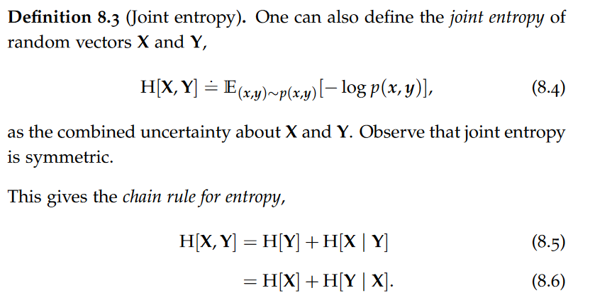
Alt text
That is, the joint entropy of X and Y is given by the uncertainty about X and the additional uncertainty about Y given X.

Mutual Information

Alt text

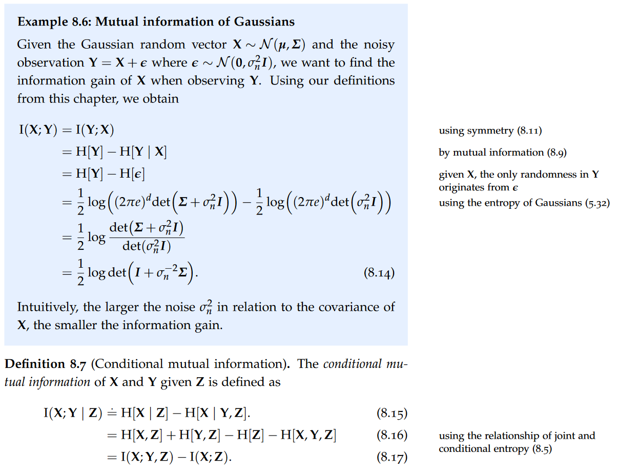
In words, we subtract the uncertainty left about X after observing Y from our initial uncertainty about X. This measures the reduction in our uncertainty in X (as measured by entropy) upon observing Y.

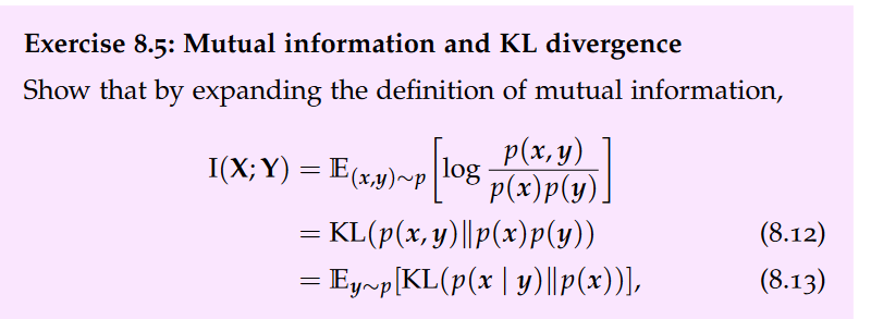
Alt text

Thus, the mutual information between X and Y can be understood as the approximation error (or information loss) when assuming that X and Y are independent.

Alt text

Thus, the conditional mutual information corresponds to the reduction of uncertainty in X when observing Y, given we already observed Z.

Following our introduction of mutual information, it is natural to answer the question “where should I collect data?” by saying “wherever mutual information is maximized”.

Submodularity of Mutual Information

Alt text

Alt text

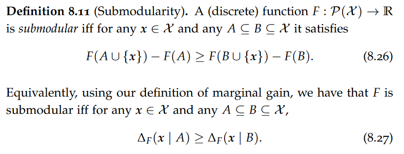
That is, “adding” x to the smaller set A yields more marginal gain than adding x to the larger set B. In other words, the function F has “diminishing returns”. In this way, submodularity can be interpreted as a notion of “concavity” for discrete functions.

Alt text

Maximizing Mutual Information

Uncertainty Sampling

Alt text

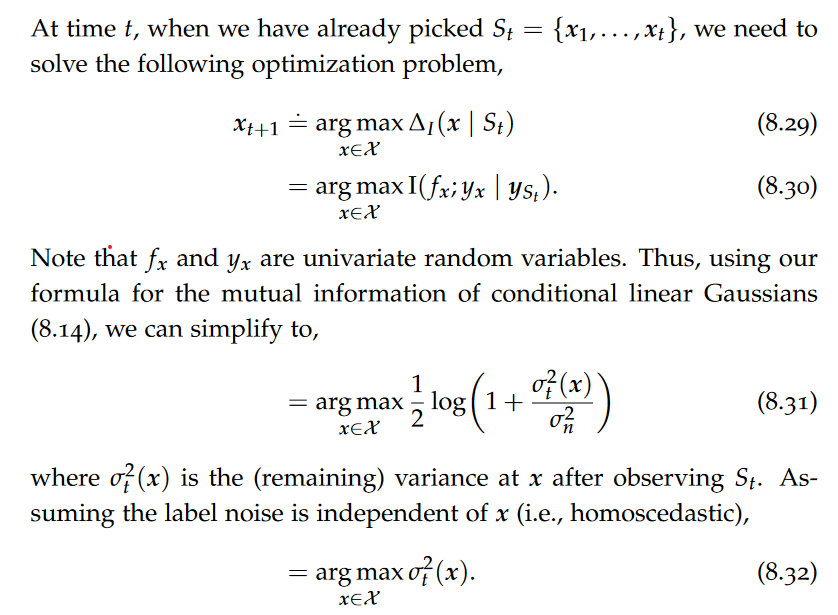
Therefore, if f is modeled by a Gaussian and we assume homoscedastic noise, greedily maximizing mutual information corresponds to simply picking the point x with the largest variance. This strategy is also called uncertainty sampling.

Heteroscedastic Noise

Uncertainty sampling is clearly problematic if the noise is heteroscedastic. If there are a particular set of inputs with a large aleatoric uncertainty dominating the epistemic uncertainty, uncertainty sampling will continuously choose those points even though the epistemic uncertainty will not be reduced substantially.
Alt text

Thus, we choose locations that trade large epistemic uncertainty with large aleatoric uncertainty. Ideally, we find a location where the epistemic uncertainty is large, and the aleatoric uncertainty is low, which promises a significant reduction of uncertainty around this location.

Classification

Here, uncertainty sampling corresponds to selecting samples that maximize the entropy of the predicted label yx.

bigdata - spark

Generic Dataflow Management

MapReduce is very simple and generic, but many more complex uses involve not just one, but a sequence of several MapReduce jobs. Furthermore, the MapReduce API is low-level, and most users need higherlevel interfaces, either in the form of APIs or query languages. This is why, after MapReduce, another generation of distributed processing technologies were invented. The most popular one is the open source Apache Spark.

A more general dataflow model

MapReduce consists of a map phase, followed by shuffling, followed by a reduce phase. In fact, the map phase and the reduce phase are not so different: both involve the computation of tasks in parallel on slots.

Resilient distributed datasets

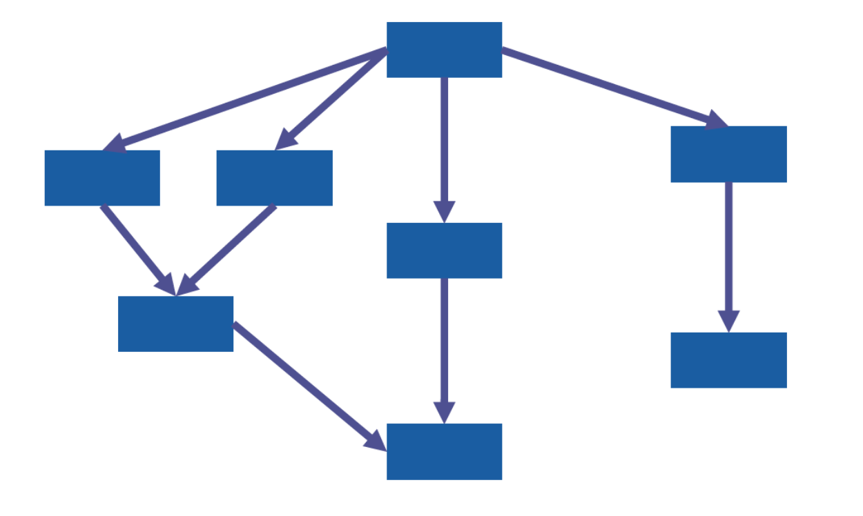
The first idea behind generic dataflow processing is to allow the dataflow to be arranged in any distributed acyclic graph (DAG).

Alt text

All the rectangular nodes in the above graph correspond to intermediate data. They are called resilient distributed datasets, or in short, RDDs.

A major difference with MapReduce, though, is that RDDs need not be collections of pairs. In fact, RDDs can be (ordered) collections of just about anything: strings, dates, integers, objects, arrays, arbitrary JSON values, XML nodes, etc.The only constraint is that the values within the same RDD share the same static type, which does not exclude the use of polymorphism.

The RDD lifecycle

Creation

RDDs undergo a lifecycle. First, they get created. RDDs can be created by reading a dataset from the local disk, or from cloud storage, or from a distributed file system, or from a database source, or directly on the fly from a list of values residing in the memory of the client using Apache Spark

Transformation

Then, RDDs can be transformed into other RDDs. Mapping or reducing, in this model, become two very specific cases of transformations. However, Spark allows for many, many more kinds of transformations. This also includes transformations with several RDDs as input.

Action

RDDs can also undergo a final action leading to making an output persistent. This can be by outputting the contents of an RDD to the local disk, to cloud storage, to a distributed file system, to a database system, or directly to the screen of the user.

Lazy evaluation

Another important aspect of the RDD lifecycle is that the evaluation is lazy: in fact, creations and transformations on their own do nothing. It is only with an action that the entire computation pipeline is put into motion, leading to the computation of all the necessary intermediate RDDs all the way down to the final output corresponding to the action.

Transformations

Unary transformations

Let us start with unary transformations, i.e., those that take a single RDD as their input.

Binary transformations

There are also transformations that take two RDDs as input.

Pair transformations

Spark has transformations specifically tailored for RDDs of key-value pairs.

Actions

Gathering output locally

The collect action downloads all values of an RDD on the client machine and outputs them as a (local) list. It is important to only call this action on an RDD that is known to be small enough (e.g., after filtering) to avoid a memory overflow.

The count action computes (in parallel) the total number of values in the input RDD. This one is safe even for RDDs with billions of values, as it returns a simple integer to the client.

Writing to sharded datasets

There is also an action called saveAsTextFile that can save the entire RDD to a sharded dataset on Cloud storage (S3, Azure blob storage) or a distributed file system (HDFS).
Binary outputs can be saved with saveAsObjectFile.

Actions on Pair RDDs

Physical architecture

Narrow-dependency transformations

In a narrow-dependency transformation, the computation of each output value involves a single input value. In a narrow-dependency transformation, the computation of each output value involves a single input value.

By default, if the transformation is applied to an RDD freshly created from reading a dataset from HDFS, each partition will correspond to an HDFS block. Thus, the computation of the narrow-dependency transformation mostly involves local reads by short-circuiting HDFS.

In fact, the way this works is quite similar to MapReduce: the sequential calls of the transformation function on each input value within a single partition is called a task. And just like MapReduce, the tasks are assigned to slots. These slots correspond to cores within YARN containers. YARN containers used by Spark are called executors. The processing of the tasks is sequential within each executor, and tasks are executed in parallel across executors. And like in MapReduce, a queue of unprocessed tasks is maintained, and everytime a slot is done, it gets a new task. When all tasks have been assigned, the slots who are done become idle and wait for all others to complete.

Chains of narrow-dependency transformations

In fact, on the physical level, the physical calls of the underlying map/filter/etc functions are directly chained on each input value to directly produce the corresponding final, output value, meaning that the intermediate RDDs are not even materialized anywhere and exist purely logically.

Such a chain of narrow-dependency transformations executed efficiently as a single set of tasks is called a stage, which would correspond to what is called a phase in MapReduce.

Physical parameters

Users can parameterize how many executors there are, how many cores there are per executor and how much memory per executor (remember that these then correspond to YARN container requests).

Shuffling

What about wide-dependency transformations? They involve a shuffling of the data over the network, so that the data necessary to compute each partition of the output RDD is physically at the same location.Thus, on the high-level of a job, the physical execution consists of a sequence of stages, with shuffling happening everytime a new stage begins.

Optimizations

Pinning RDDs

Everytime an action is triggered, all the computations of the ”reverse transitive closure” (i.e., all the way up the DAG through the reverted edges) are set into motion. In some cases, several actions might share subgraphs of the DAG. It makes sense, then, to “pin” the intermediate RDD by persisting it.

Pre-partitioning

Shuffle is needed to bring together the data that is needed to jointly contribute to individual output values. If, however, Spark knows that the data is already located where it should be, then shuffling is not needed.

DataFrames in Spark

Data independence

Unlike a relational database that has everything right off-theshelf, with RDDs, the user has to re-implement all the primitives they need. This is a breach of the data independence principle. The developers behind Spark addressed this issue in a subsequent version of Spark by extending the model with support for DataFrames and Spark SQL, bringing back a widely established and popular declarative, high-level language into the ecosystem.

A specific kind of RDD

A DataFrame can be seen as a specific kind of RDD: it is an RDD of rows (equivalently: tuples, records) that has relational integrity, domain integrity, but not necessarily atomic integrity.

Performance impact

DataFrames are stored column-wise in memory, meaning that the values that belong to the same column are stored together. Furthermore, since there is a known schema, the names of the attributes need not be repeated in every single row, as would be the case with raw RDDs. DataFrames are thus considerably more compact in memory than raw RDDs.

Generally, Spark converts Spark SQL to internal DataFrame transformation and eventually to a physical query plan. An optimizer known as Catalyst is then able to find many ways of making the execution faster.

Input formats

Note that Spark automatically infers the schema from discovering the JSON Lines file, which adds a static performance overhead that does not exist for raw RDDs.

DataFrame transformations

It is also possible, instead of Spark SQL, to use a transformation API similar to (but distinct from) the RDD transformation API.

Unlike the RDD transformation API, there is no guarantee that the execution will happen as written, as the optimizer is free to reorganize the actual computations.

DataFrame column types

DataFrames also support the three structured types: arrays, structs, and maps. As a reminder, structs have string keys and arbitrary value types and correspond to generic JSON objects, while in maps, all values have the same type. Thus, structs are more common than maps.

The Spark SQL dialect

Note that both GROUP BY and ORDER BY will trigger a shuffle in the system, even though this can be optimized as the grouping key and the sorting key are the same. The SORT BY clause can sort rows within each partition, but not across partitions, i.e., does not induce any shuffling. The DISTRIBUTE BY clause forces a repartition by putting all rows with the same value (for the specified field(s)) into the same new partition.
Note that the SORT BY clause is used to return the result rows sorted within each partition in the user specified order. When there is more than one partition SORT BY may return result that is partially ordered. This is different than ORDER BY clause which guarantees a total order of the output.

A word of warning must be given on SORT, DISTRIBUTE and CLUSTER clauses: they are, in fact, a breach of data independence, because they expose partitions.

Spark SQL also comes with language features to deal with nested arrays and objects. First, nested arrays can be navigated with the explode() function. Lateral views are more powerful and generic than just an explode() because they give more control, and they can also be used to go down several levels of nesting. A lateral view can be intuitively described this way: the array mentioned in the LATERAL VIEW clause is turned into a second, virtual table with the rest of the original table is joined. The other clauses can then refer to columns in both the original and second, virtual table.

exercise

RDD

Why RDD should be immutable and lazy: immutable is for lineage.
Why need RDD partitioning: parallel computing and reduce shuffling.

DataFrame API

For nested array,use array_contains.

spark SQL

In jupyter notebook, we can use “%load_ext sparksql_magic” directly.

reference

https://www.analyticsvidhya.com/blog/2016/10/spark-dataframe-and-operations/

Probabilistic Artificial Intelligence - Bayesian Deep Learning

SWAG(Stochastic Weight Averaging Gaussian)

This paper proposes a different approach to Bayesian deep learning: they use the information contained in the SGD trajectory to efficiently approximate the posterior distribution over the weights of the neural network [1].

SWA

This paper shows that simple averaging of multiple points along the trajectory of SGD, with a cyclical or constant learning rate, leads to better generalization than conventional training [2].

cyclical learning rate schedule

Calibration of Modern Neural Networks

Confidence calibration – the problem of predicting probability estimates representative of the true correctness likelihood – is important for classification models in many applications. Through extensive experiments, we observe that depth, width, weight decay, and Batch Normalization are important factors influencing calibration.

references

[1] Maddox W J, Izmailov P, Garipov T, et al. A simple baseline for bayesian uncertainty in deep learning[J]. Advances in neural information processing systems, 2019, 32.
[2] Izmailov P, Podoprikhin D, Garipov T, et al. Averaging weights leads to wider optima and better generalization[J]. arXiv preprint arXiv:1803.05407, 2018.
[3] Guo C, Pleiss G, Sun Y, et al. On calibration of modern neural networks[C]//International conference on machine learning. PMLR, 2017: 1321-1330.

bigdata - YARN

Resource management

The first version of MapReduce is inefficient in several respects. For this reason, the architecture was fundamentally changed by adding a resource management layer to the stack, adding one more level of decoupling between scheduling and monitoring. A resource management system, here YARN, is a very important building block not only for a better MapReduce, but also for many other technologies running on a cluster.

Limitations of MapReduce in its first version

The JobTracker has a lot on its shoulders! It has to deal with resource management, scheduling, monitoring, the job lifecycle, and fault tolerance.The first consequence of this is scalability. The second consequence is the bottleneck that this introduces at the JobTracker level, which slows down the entire system. The third issue is that it is difficult to design a system that do many things well. The fourth issue is that resources are statically allocated to the Map or the Reduce phase, meaning that parts of the cluster remain idle during both phases. The fifth issue is the lack of fungibility between the Map phase and the Reduce phase.

YARN

General architecture

YARN means Yet Another Resource manager. It was introduced as an additional layer that specifically handles the management of CPU and memory resources in the cluster.

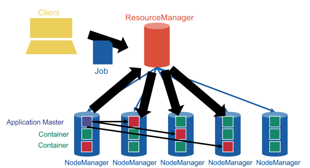
YARN, unsurprisingly, is based on a centralized architecture in which the coordinator node is called the ResourceManager, and the worker nodes are called NodeManagers. NodeManagers furthermore provide slots (equipped with exclusively allocated CPU and memory) known as containers.

When a new application is launched, the ResourceManager assigns one of the container to act as the ApplicationMaster which will take care of running the application. The ApplicationMaster can then communicate with the ResourceManager in order to book and use more containers in order to run jobs. This is a fundamental change from the initial MapReduce architecture, in which the JobTracker was also taking care of running the MapReduce job.

Alt text

Thus, YARN cleanly separates between the general management of resources and bootstrapping new applications, which remains centralized on the coordinator node, and monitoring the job lifecycle, which is now delegated to one or more ApplicationMasters running concurrently. This means, in particular, that several applications can run concurrently in the same cluster. This ability, known as multi-tenancy, is very important for large companies or universities in order to optimize the use of their resources.

Resource management

In resource management, one abstracts away from hardware by distinguish between four specific resources used in a distributed database system. These four resources are: • Memory • CPU • Disk I/O • Network I/O.
ApplicationMasters can request and release containers at any time, dynamically. A container request is typically made by the ApplicationMasters with a specific demand. If the request is granted by the ResourceManager fully or partially, this is done indirectly by signing and issuing a container token to the ApplicationMaster that acts as proof that the resource was granted. The ApplicationMaster can then connect to the allocated NodeManager and send the token. The NodeManager will then check the validity of the token and provide the memory and CPU granted by the ResourceManager. The ApplicationMaster ships the code (e.g., as a jar file) as well as parameters, which then runs as a process with exclusive use of this memory and CPU.

Job lifecycle management and fault tolerance

Version 2 of MapReduce works on top of YARN by leaving the job lifecycle management to an ApplicationMaster. The ApplicationMaster requests containers for the Map phase, and sets these containers up to execute Map tasks. As soon as a container is done executing a Map task, the ApplicationMaster will assign a new Map task to this container from the remaining queue, until no Map tasks are left.

a container in the Map phase can contain several Map slots. Sharing memory and containers across slots in this way improves the overall efficiency, because setting up a container adds latency. It is thus more efficient to allocate 10 containers of each 4 cores, compared to 40 containers of each 1 core.

In the event of a container crashing during the Map phase, the ApplicationMaster will handle this by re-requesting containers and restarting the failed tasks. In the case that some data is lost in the Reduce phase, it is possible that the entire job must be restarted, because this the only way to recreate the intermediate data is to re-execute the Map tasks.

Scheduling

The ResourceManager keeps track of the list of available NodeManagers (who can dynamically come and go) and their status. Just like in HDFS, NodeManagers send periodic heartbeats to the ResourceManager to give a sign of life. The ResourceManager also offers an interface so that ApplicationMasters can register and send container requests. ApplicationMasters also send periodic heartbeats to the ResourceManager. It is important to understand that, unlike the JobTracker, the ResourceManager does not monitor tasks, and will not restart slots upon failure. This job is left to the ApplicationMasters.

Scheduling strategies

FIFO scheduling

In FIFO scheduling, there is one application at a time running on the entire cluster. When it is done, the next application runs again on the entire cluster, and so on.

Capacity scheduling

In capacity scheduling, the resources of the cluster are partitioned into several sub-clusters of various sizes. Each one of these sub-clusters has its own queue of applications running in a FIFO fashion within this queue. Capacity scheduling also exists in a more “dynamic flavour” in which, when a sub-cluster is not currently used, its resources can be temporarily lent to the other sub-clusters. This is also in the spirit of usage maximization.

Fair scheduling

Fair scheduling involves more complex algorithms that attempt to allocate resources in a way fair to all users of the cluster and based on the share they are normally entitled to. fair scheduling consists on making dynamic decisions regarding which requests get granted and which requests have to wait. Fair scheduling combines several ways to compute cluster shares: Steady fair share: this is the share of the cluster officially allocated to each department. Instantaneous fair share: this is the fair share that a department should ideally be allocated (according to economic and game theory considerations) at any point in time. This is a dynamic number that changes constantly, based on departments being idle: if a department is idle, then the instantaneous fair share of others department becomes higher than their steady fair shares. Current share: this is the actual share of the cluster that a department effectively uses at any point in time. This is highly dynamic. The current share does not necessarily match the instantaneous fair share because there is some inertia in the process: a department might be using more resources while another is idle. When the other department later stops being idle, these resources are not immediately withdrawn from the first department; rather, the first department will stop getting more resources, and the second department will gradually recover these resources as they get released by the first department.

The easiest case of fair scheduling is when only one resource is considered: for example, only CPU cores, or only memory. Things become more complicated when several resources are considered, in practice both CPU cores and memory. This problem was solved game-theoretically with the Dominant Resource Fairness algorithm. The two (or more) dimensions are projected again to a single dimension by looking at the dominant resource for each user.

exercise

motivation

improve hadoop 1.x by adding a layer YARN to separate resource management from data processing.

architecture

NodeMananger is generalized taskTracker.
On ResourceManager, there is an ApplicationManager rsponsible for admiting new jobs and collecting finished jobs and logs.
A scheduler has a global view to assign an ApplicationMaster. The applicationMaster will compute how many resources needed and send a request to the scheduler.

fault tolerance is provided by applicationMaster+NodeManager+HDFS.

bigdata - Map Reduce

Patterns of large-scale query processing

Textual input

We saw that the data we want to query can take many forms. First, it can be billions of lines of text. It can also be plenty of CSV lines. Some other formats (e.g., Parquet, …) can be binary. We also encountered HFiles in Chapter 6, which are lists of keyvalue pairs. In fact, Hadoop has another such kind of key-value-based format called Sequence File, which is simply a list of key-values, but not necessarily sorted by key (although ordered) and with keys not necessarily unique.

Shards

There are several practical motivations for the many-files pattern even in HDFS.

Querying pattern

This is the motivation behind the standard MapReduce pattern: a map-like phase on the entire input, then a shuffle phase on the intermediate data, then another map-like phase (called reduce) producing the entire output

MapReduce Model

In MapReduce, the input data, intermediate data, and output data are all made of a large collection of key-value pairs (with the keys not necessarily unique, and not necessarily sorted by key). The types of the keys and values are known at compile-time (statically), and they do not need to be the same across all three collections.

MapReduce architecture

On a cluster, the architecture is centralized, just like for HDFS and HBase. In the original version of MapReduce, the main node is called JobTracker, and the worker nodes are called TaskTrackers.

In fact, the JobTracker typically runs on the same machine as the NameNode (and HMaster) and the TaskTrackers on the same machines as the DataNodes (and RegionServers). This is called “bring the query to the data.”

As the map phase progresses, there is a risk that the memory becomes full. But we have seen this before with HBase: the intermediate pairs on that machine are then sorted by key and flushed to the disk to a Sequence File. And as more flushes happen, these Sequence Files can be compacted to less of them, very similarly to HBase’s Log-Structured Merge Trees. When the map phase is over, each TaskTracker runs an HTTP server listening for connections, so that they can connect to each other and ship the intermediate data over to create the intermediate partitions ensuring that the same keys are on the same machines.This is the phase called shuffling. Then, the reduce phase can start. When the reduce phase is completed, each output partition will be output to a shard (as we saw, a file named incrementally) in the output destination (HDFS, S3, etc) and in the desired format.

Note that shuffling can start before the map phase is over, but the reduce phase can only start after the map phase is over.

MapReduce input and output formats

Impedance mismatch

MapReduce can read its input from files lying in a data lake as well as directly from a database system such as HBase or a relational database management system. MapReduce only reads and writes lists of key-value pairs, where keys may be duplicates and need not appear in order. However, the inputs we considered are not key-value pairs. So we need an additional mechanism that allows MapReduce to interpret this input as key-value pairs. For tables, whereas relational or in a wide column stores, this is relatively easy: indeed, tables have primary keys, consisting of either a single column or multiple columns. Thus, each tuple can be interpreted as a key-value pair.

Mapping files to pairs

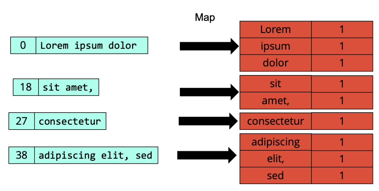
How do we read a (possibly huge) text file as a list of key-value pairs? The most natural way to do so is to turn each line of text in a key value pair1: the value is the string corresponding to the entire line, while the key is an integer that expresses the position (as a number of characters), or offset, at which the line starts in the current file being read.

A few examples

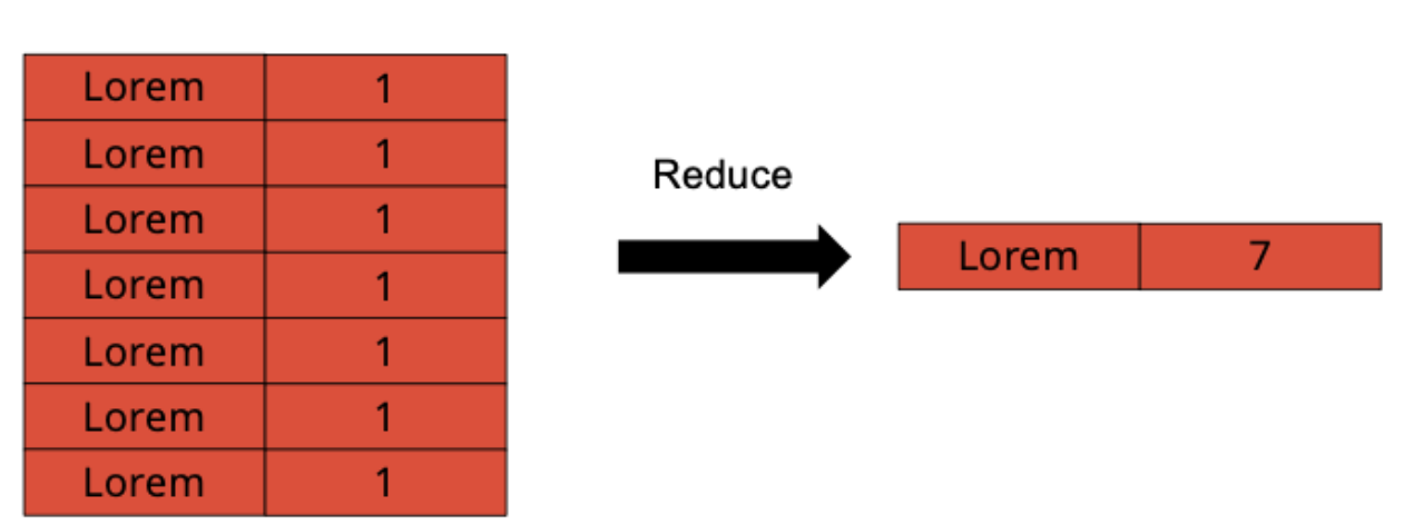
Counting words

Alt text
Alt text

Selecting

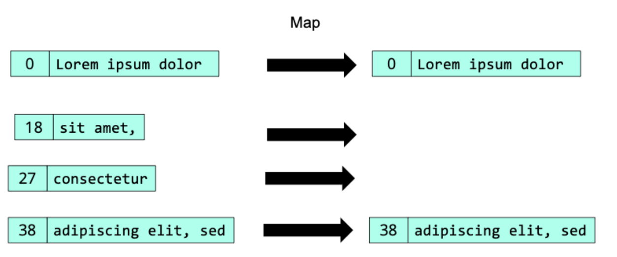
This is something easily done by having a map function that outputs a subset of its input, based on some predicate provided by the user.
Alt text
Here we notice that the output of the map phase already gives us the desired result; we still need to provide a reduce function, which is taken trivially as the identity function. This is not unusual (and there are also examples where the map function is trivial, and the reduce function is doing the actual processing).

Projecting

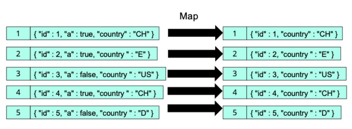
The map function can project this object to an object with less attributes:
Alt text

MapReduce and the relational algebra

As an exercise, try to figure out how to implement a GROUP BY clause and an ORDER BY clause. What about the HAVING clause? Naturally, executing these queries directly in MapReduce is very cumbersome because of the low-level code we need to write.

Combine functions and optimization

In addition to the map function and the reduce function, the user can supply a combine function. This combine function can then be called by the system during the map phase as many times as it sees fit to “compress” the intermediate key-value pairs. Strategically, the combine function is likely to be called at every flush of key-value pairs to a Sequence File on disk, and at every compaction of several Sequence Files into one.

However, there is no guarantee that the combine function will be called at all, and there is also no guarantee on how many times it will be called. Thus, if the user provides a combine function, it is important that they think carefully about a combine function that does not affect the correctness of the output data.

In fact, in most of the cases, the combine function will be identical to the reduce function, which is generally possible if the intermediate key-value pairs have the same type as the output key-value pairs, and the reduce function is both associative and commutative.

MapReduce programming API

Mapper classes

In Java, the user needs to define a so-called Mapper class that contains the map function, and a Reducer class that contains the reduce function. A map function takes in particular a key and a value. Note that it outputs key-value pairs via the call of the write method on the context, rather than with a return statement.

Reducer classes

A reduce function takes in particular a key and a list of values. Note that it outputs key-value pairs via the call of the write method on the context, rather than with a return statement.

Running the job

Finally, a MapReduce job can be created and invoked by supplying a Mapper and Reducer instance to the job. A combine function can also be supplied with the setCombinerClass method. It is also possible to use Python rather than Java, via the socalled Streaming API. The Streaming API is the general way to invoke MapReduce jobs in other languages than Java.

Using correct terminology

Functions

A map function is a mathematical, or programmed, function that takes one input key-value pair and returns zero, one or more intermediate key-value pairs.

A reduce function is a mathematical, or programmed, function that takes one or more intermediate key-value pairs and returns zero, one or more output key-value pairs.

A combine function is a mathematical, or programmed, function that takes one or more intermediate key-value pairs and returns zero, one or more intermediate key-value pairs.

Note that the combine function is an optional local aggregation step that occurs before shuffling and sorting, and its purpose is to reduce the amount of data that needs to be transferred to the reducers. The reduce function, on the other hand, performs the final aggregation and processing based on keys.

Tasks

A map task is an assignment (or “homework”, or “TODO”) that consists in a (sequential) series of calls of the map function on a subset of the input.

A reduce task is an assignment that consists in a (sequential) series of calls of the reduce function on a subset of the intermediate input.

We insist that the calls within a task are sequential, meaning that there is no parallelism at all within a task.

There is no such thing as a combine task. Calls of the combine function are not planned as a task, but is called ad-hoc during flushing and compaction.

Slots

The map tasks are processed thanks to compute and memory resources (CPU and RAM). These resources are called map slots. One map slot corresponds to one CPU core and some allocated memory. The number of map slots is limited by the number of available cores. Each map slot then processes one map task at a time, sequentially. The resources used to process reduce tasks are called reduce slots. So, there is no parallelism either within one map slot, or one reduce slot. In fact, parallelism happens across several slots.

Phases

The map phase thus consists of several map slots processing map tasks in parallel.

blocks vs. splits

HDFS blocks have a size of (at most) 128 MB. In every file, all blocks but the last one have a size of exactly 128 MB. Splits, however, only contain full records: a key-value pair will only belong to one split (and thus be processed by one map task).

Probabilistic Artificial Intelligence - Markov Chain Monte Carlo Methods

Markov Chain Monte Carlo Methods

The key idea of Markov chain Monte Carlo methods is to construct a Markov chain, which is efficient to simulate and has the stationary distribution p.

Markov Chains

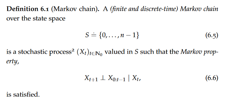
Alt text

Intuitively, the Markov property states that future behavior is independent of past states given the present state.

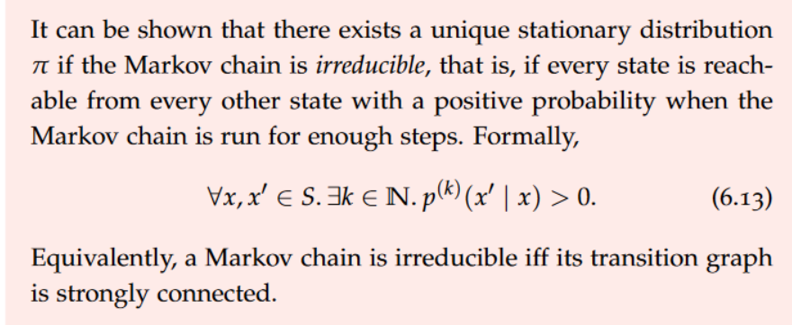
Markov chains can be classified into different types based on their behavior. These classifications include time-homogeneous and time-inhomogeneous Markov chains, irreducible Markov chains, and periodic and aperiodic Markov chains.

We restrict our attention to time-homogeneous Markov chains. That is, the transition probabilities do not change over time, which can be characterized by a transition function.

Irreducible Markov chains are those in which every state can be reached from any other state, while periodic Markov chains exhibit a repeating pattern in their states. On the other hand, aperiodic Markov chains do not exhibit any regular pattern in their states. If there is no fixed period at which the probabilities return to the starting values, the chain is classified as aperiodic. Aperiodic Markov chains often display a more complex and unpredictable behavior compared to periodic ones.

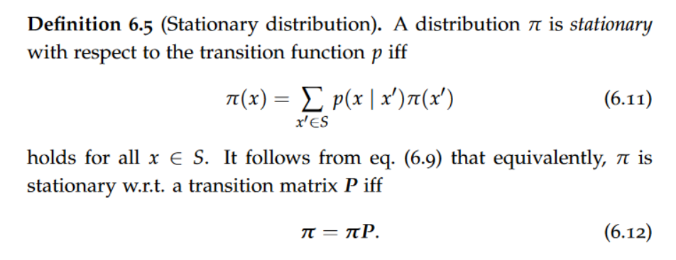
Stationarity

Alt text

Alt text

Convergence

Alt text

Alt text

Alt text

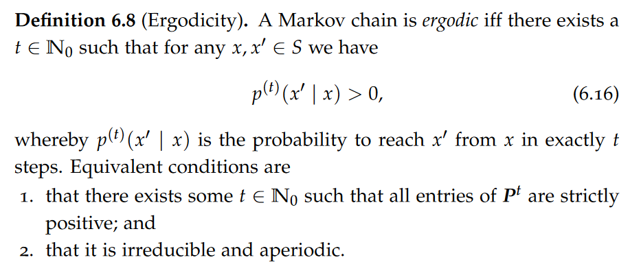
A Markov Chain is called ergodic, if there exists a finite t such that every state can be reached from every state in exactly t steps.

Fundamental theorem of ergodic Markov chains

Alt text

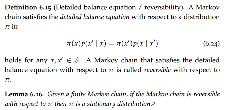
Detailed Balance Equation

Alt text

Ergodic Theorem

Alt text

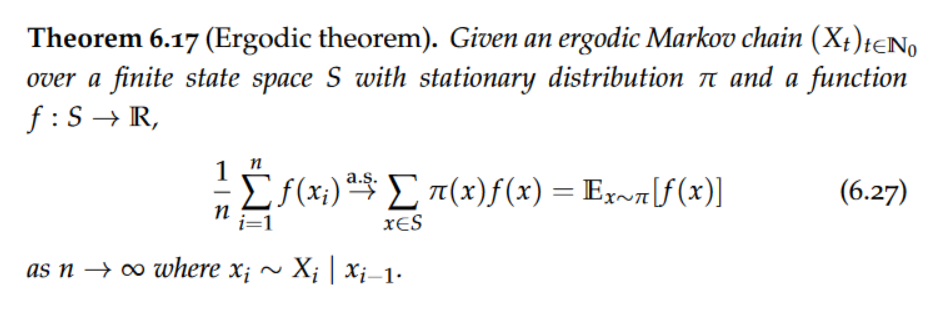
This result is the fundamental reason for why Markov chain Monte Carlo methods are possible. In practice, one observes that Markov chain Monte Carlo methods have a so-called “burn-in” time during which the distribution of the Markov chain does not yet approximate the posterior distribution well. Typically, the first t0 samples are therefore discarded. It is not clear in general how T and t0 should be chosen such that the estimator is unbiased, rather they have to be tuned.

Elementary Sampling Methods

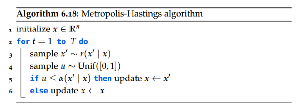
Metropolis-Hastings Algorithm

Alt text

Gibbs Sampling

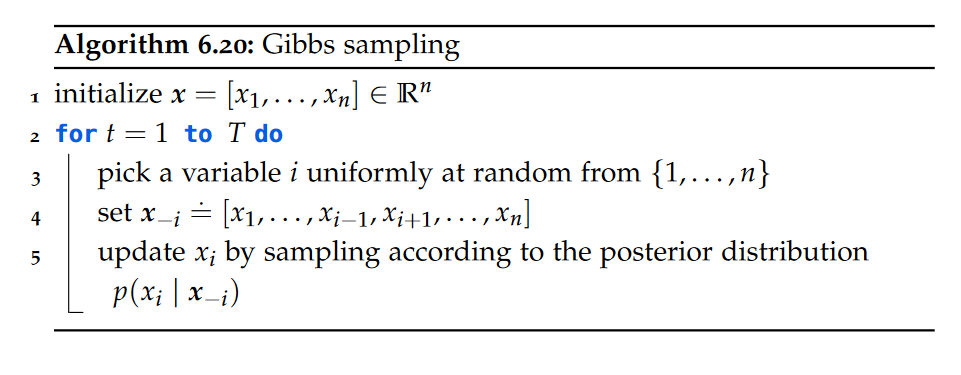
A popular example of a Metropolis-Hastings algorithm is Gibbs sampling.

Alt text

Intuitively, by re-sampling single coordinates according to the posterior distribution given the other coordinates, Gibbs sampling finds states that are successively “more” likely.

Langevin Dynamics

Gibbs Distributions

references

https://www.collimator.ai/reference-guides/what-is-a-aperiodic-markov-chain

bigdata - data model

data model

A data model is an abstract view over the data that hides the way it is stored physically.

The JSON Information Set

The appropriate abstraction for any JSON document is a tree. The nodes of that tree, which are JSON logical values, are naturally of six possible kinds: the six syntactic building blocks of JSON.

These are the four leaves corresponding to atomic values:Strings, Numbers,Booleans, Nulls. As well as two intermediate nodes: Objects, Arrays. These nodes are generally called information items and form the logical building blocks of the model, called information set.

The XML Information Set

A fundamental difference between JSON trees and XML trees is that for JSON, the labels (object keys) are on the edges connecting an object information item to each one of its children information items. In XML, the labels (these would be element and attribute names) are on the nodes (information items) directly.

In XML, there are many more information items: Document information items, Element, Attribute, Character, Comment, Processing instruction, Name space, Unexpanded entity reference, DTD, Unparsed entity, Notation. Here we only focus on documents, elements, attributes, and characters.

Validation

Once documents, JSON or XML, have been parsed and logically abstracted as a tree in memory, the natural next step is to check for further structural constraints.

In a relational database, the schema of a table is defined before any data is populated into the table. Thus, the data in the table is guaranteed, at all times, to fulfil all the constraints of the schema. The schema was enforced at write time (schema on write). A collection of JSON and XML documents out there can exist without any schema and contain arbitrary structures. Validation happens “ex post,” that is, only after reading the data (schema on read).

JSON and XML documents undergo two steps: a well-formedness check: attempt to parse the document and construct a tree representation in memory;(if the first step succeeded) a validation check given a specific schema. Note that, unlike well-formedness, validation is schema dependent: a given well-formed document can be valid against schema A and invalid against schema B.

Item types

A fundamental aspect of validation is the type system. A well-designed type system, in turn, allows for storing the data in much more efficient, binary formats tailored to the model.

Atomic types

Atomic types correspond to the leaf of a tree data model: these are types that do not contain any further nestedness. The kinds of atomic types available are also relatively standard and common to most technologies. Also, all atomic types have in common that they have a logical value space and a lexical value space.

An atomic type also has a (not necessarily injective) mapping from its lexical value space to its logical value space (e.g., mapping the hexadecimal literal x10 to the mathematical integer sixteen).
Atomic types can be in a subtype relationship: a type is a subtype of another type if its logical value space is a subset of the latter.

Strings

In “pure computer science” textbooks, strings are often presented as structured values rather than as atomic values because of their complexity on the physical layer. However, for us data scientists, strings are atomic values.

Numbers: integers

Integers correspond to finite cardinalities (counting) as well as their negative counterparts. In older programming languages, support for integers used to be bounded. However, in modern databases, it is customary to support unbounded integers. Engines can optimize computations for small integers, but might become less efficient with very large integers.

Numbers: decimals

Decimals correspond to real numbers that can be written as a finite sequence of digits in base 10, with an optional decimal period.

Numbers: floating-point

Support for the entire decimal value space can be costly in performance. In order to address this issue, a floating-point standard (IEEE 754) was invented and is still very popular today.

Floating-point numbers are limited both in precision and magnitude (both upper and lower) in order to fit on 32 bits (float) or 64 bits (double). Floats have about 7 digits of precision and their absolute value can be between roughly 10^−37 and 10^37, while doubles have 15 digits of precision and their absolute value can be between roughly 10^−307 and 10^308.

Booleans

The logical value space for the Boolean type is made of two values: true and false as in NoSQL queries, two-valued logic is typically assumed.

Dates and times

Dates are commonly using the Gregorian calendar (with some technologies possibly supporting more) with a year (BC or AD), a month and a day of the month. Times are expressed in the hexagesimal (60) basis with hours, minutes, seconds, where the seconds commonly go all the way to microseconds (six digits after the decimal period). Datetimes are expressed with a year, a month, a day of the month, hours, minutes and (decimal) seconds.

Timestamp values are typically stored as longs (64-bit integers) expressing the number of milliseconds elapsed since January 1, 1970 by convention.

XML Schema, JSound and JSONiq follow the ISO 8601 standard, where lexical values look like so (with many parts optional): 2022-08-07T14:18:00.123456+02:00.

Durations

The lexical representation can vary, but there is a standard defined by ISO 8601 as well, starting with a P and prefixing sub-day parts with a T.
4 days, 3 hours, 2 minutes and 1.123456 seconds: P4DT3H2M1.123456S.

Binary data

Binary data is, logically, simply a sequence of bytes. There are two main lexical representations used in data: hexadecimal and base64. Hexadecimal expresses the data with two hexadecimal digits per byte. Base 64, formally, does the same but in the base 64, which “wastes” less lexical space in the text. It does so by encoding the bits six by six, encoding each sequence of six bits with one base-64 digit.

Null

A schema can either allow, or disallow the null value.
XML also supports null values, but calls them “nil” and does so with a special attribute and no content rather than with a lexical representation

Structured types

Lists

Lists correspond to JSON arrays and are ordered sequences of (atomic or structured) values.

Records

Records, or structs, correspond to JSON objects and are maps from strings to values.

Maps

Maps (not be confused with records, which are similar) are maps from any atomic value to any value, i.e., generalize objects to keys that are not necessarily strings (e.g., numbers, dates, etc).
With a schema, it is possible to restrict the type of the keys, as well as the type of the values. However, unlike records, the type of the values must be the same for all keys.

Sets

Sets are like lists, but without any specific ordering, and without duplicate values.

XML elements and attributes

XML Schema stands apart from most other technologies and formats, in that it does not offer specific support for records and maps; it offers some limited support for lists, but considers them to be simple types, which are “inbetween” atomic types and structured types. n XML Schema, structure is obtained, instead, with elements and attributes, and the machinery for elements and attributes is highly specific to XML.

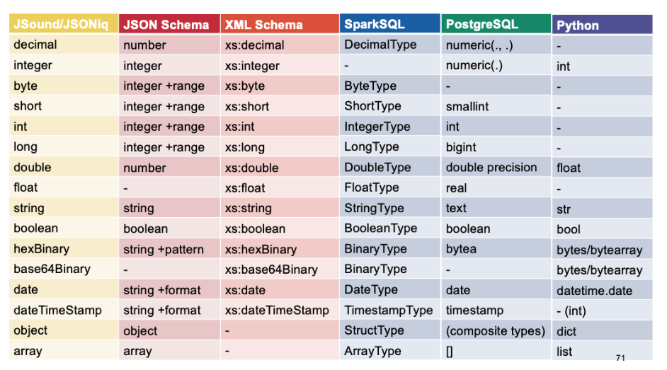
Type names
Alt text

Sequence types

Cardinality

Many type system give options regarding the number of occurrences of items in a sequence.

Collections vs. nested lists

A collection of items is on the outer level, and can be massively large (billions, trillions of items).

A list (or array) of items, however, usually refers to a nested structure, for example an array nested inside a document or object. Such lists of items are usually restricted in size for reasons of performance and scalability.

It is thus important to keep this subtle difference in mind, in particular, do not confuse a collection of integers with a collection that contains a single array of integers.

JSON validation

Validating flat objects

JSound is a schema language that was designed to be simple for 80% of the cases, making it particularly suitable in a teaching environment.It is independent of any programming language.JSON Schema is another technology for validating JSON documents. The available JSON Schema types are string, number, integer, boolean, null, array and object.

An example for a json document is like:
{ “name” : “Einstein”, “first” : “Albert”, “age” : 142 }
The JSound and the JSON Schema are as follows:
{ “name” : “string”, “first” : “string”, “age” : “integer” }

{ “type” : “object”, “properties” : { “name” : “string”, “first” : “string”, “age” : “number” } }.

The type system of JSON Schema is thus less rich than that of JSound, but extra checks can be done with so-called formats, which include date, time, duration, email, and so on including generic regular expressions.

Requiring the presence of a key

It is possible to require the presence of a key by adding an exclamation mark in JSound. The equivalent JSON Schema uses a “required” property associated with the list of required keys to express the same.

Open and closed object types

In the JSound compact syntax, extra keys are forbidden. The schema is said to be closed. There are ways to define JSound schemas to allow arbitrary additional keys (open schemas), with a more verbose syntax. Unlike JSound, in JSON Schema, extra properties are allowed by default. JSON Schema then allows to forbid extra properties with the “additionalProperties” property.

Nested structures

{ “numbers” : [ “integer” ] }
Every schema can be given a name, turning into a type.
JSound allows for the definition not only of arbitrary array and object types, but also user-defined types.

Primary key constraints, allowing for null, default values

There are a few more features available in the compact JSound syntax (not in JSON Schema) with the special characters @, ? and =. The question mark (?) allows for null values. The arobase (@) indicates that one or more fields are primary keys for a list of objects that are members of the same array. The equal sign (=) is used to indicate a default value that is automatically populated if the value is absent.

Note that validation only checks whether lexical values are part of the type’s lexical space.

Accepting any values

Accepting any values in JSound can be done with the type “item”, which contains all possible values. In JSON Schema, in order to declare a field to accept any values, you can use either true or an empty object in lieu of the type. JSON Schema additionally allows to use false to forbid a field.

Type unions

In JSON Schema, it is also possible to combine validation checks with Boolean combinations. JSound schema allows defining unions of types with the vertical bar inside type strings, like so: “string|array”.

Type conjunction, exclusive or, negation

In JSON Schema only (not in JSound), it is also possible to do a conjunction (logical and), as well as exclusive or (xor), as well as negation.

XML validation

Simple types

All elements in an XML Schema are in a namespace, the XML Schema namespace. It is recommended to stick to the prefix xs, or xsd, which is also quite popular. We do not recommend declaring the XML Schema namespace as a default namespace, because it can create confusion in several respects.

The list of predefined atomic types is the same as in JSound, except that in XML Schema, all these predefined types live in the XML Schema namespace and thus bear the prefix xs as well.

Builtin types

XML Schema allows you to define user-defined atomic types, for example restricting the length of a string to 3 for airport codes, and then use it with an element.

Complex types

It is also possible to constrain structures and the element/attribute/text hierarchy with complex types applying to element nodes.
There are four main kinds of complex types:• complex content: there can be nested elements, but there can be no text nodes as direct children. • simple content: there are no nested elements: just text, but attributes are also possible. • empty content: there are neither nested elements nor text, but attributes are also possible. • mixed content: there can be nested elements and it can be intermixed with text as well.

Attribute declarations

Finally, all types of content can additionally contain attributes. Attributes always have a simple type.

Anonymous types

Finally, it is not mandatory to give a name to all types. Be careful: if there is neither a type attribute nor a nested type declaration, then anything is allowed!

Miscellaneous

Finally, XML Schema documents are themselves XML documents, and can thus be validated against a “schema or schemas”, itself written as an XML Schema.This schema has the wonderful property of being valid against itself.

Data frames

Heterogeneous, nested datasets

The beauty of the JSON data model is that, unlike the relational model and the CSV syntax, it supports nested, heterogeneous datasets, while also supporting as a particular case flat, homogeneous datasets.

Dataframe visuals

There is a particular subclass of semi-structured datasets that are very interesting: valid datasets, which are collections of JSON objects valid against a common schema, with some requirements on the considered schemas. The datasets belonging to this particular subclass are called data frames, or dataframes.

Specifically, for the dataset to qualify as a data frame, firstly, we forbid schemas that allow for open object types. secondly, we forbid schemas that allow for object or array values to be too permissive and allow any values. We, however, include schemas that allow for null values and/or absent values. Relational tables are data frames, while data frames are not necessarily relational tables. Data frames are a generalization of (normalized) relational tables allowing for (organized and structured) nestedness.

exercies

complextType cannot contain character by default but with mixed=”true” it can.

protobuf

convert json-like data to columnar representation(why we want this: make it more efficient to get relevant data rather than get the whole table).

convert the columnar representation back to the original format. Replace the missing field with NULL. It’s a “lossless” conversion.

Dremel

optional: 0 or 1. repeated: 1 or more.
Probabilistic Artificial Intelligence - Variational Inference

Variational Inference

The fundamental idea behind variational inference is to approximate the true posterior distribution using a “simpler” posterior that is as close as possible to the true posterior.

where λ represents the parameters of the variational posterior q, also called variational parameters.

Laplace Approximation

A natural idea for approximating the posterior distribution is to use a Gaussian approximation (that is, a second-order Taylor approximation) around the mode of the posterior. Such an approximation is known as a Laplace approximation.

As an example, we will look at Laplace approximation in the context of Bayesian logistic regression. Bayesian logistic regression corresponds to Bayesian linear regression with a Bernoulli likelihood.

Intuitively, the Laplace approximation matches the shape of the true posterior around its mode but may not represent it accurately elsewhere — often leading to extremely overconfident predictions.

Inference with a Variational

Information Theory

Surprise

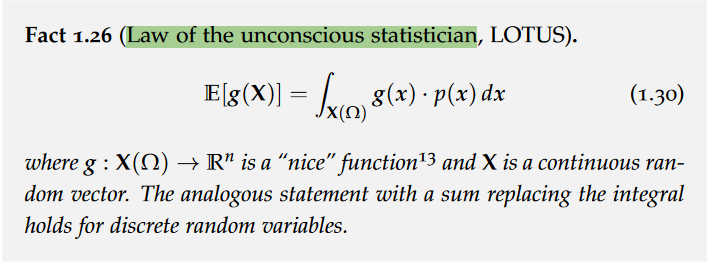
The surprise about an event with probability u is defined as $S[u] = -log u$.
Alt text

Entropy

The entropy of a distribution p is the average surprise about samples from p.if the entropy of p is large, we are more uncertain about x ∼ p than if the entropy of p were low.

Cross-Entropy

Alt text
Cross-entropy can also be expressed in terms of the KL-divergence. Quite intuitively, the average surprise in samples from p with respect to the distribution q is given by the inherent uncertainty in p and the additional surprise that is due to us assuming the wrong data distribution q. The “closer” q is to the true data distribution p, the smaller is the additional average surprise.
Variational Families

We can view variational inference more generally as a family of approaches aiming to approximate the true posterior distribution by one that is closest (according to some criterion) among a “simpler” class of distributions.
Alt text

Kullback-Leibler Divergence

Alt text

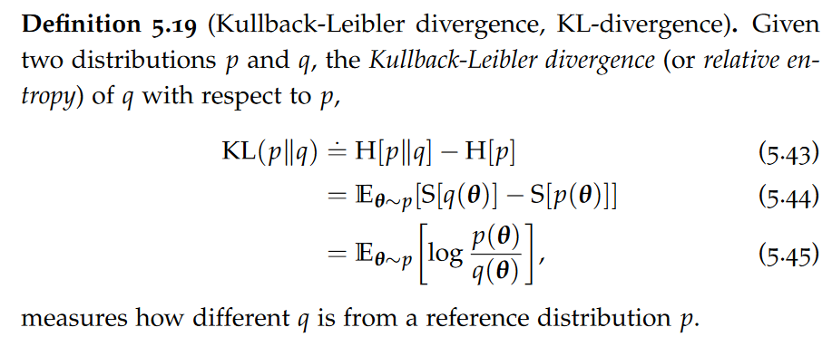
In words, KL(p∥q) measures the additional expected surprise when observing samples from p that is due to assuming the (wrong) distribution q and which not inherent in the distribution p already. Intuitively, the KL-divergence measures the information loss when approximating p with q.
Alt text

Forward and reverse KL-divergence

KL(p∥q) is also called the forward (or inclusive) KL-divergence. In contrast, KL(q∥p) is called the reverse (or exclusive) KL-divergence.

It can be seen that the reverse KL-divergence tends to greedily select the mode and underestimating the variance which, in this case, leads to an overconfident prediction. The forward KL-divergence, in contrast, is more conservative and yields what one could consider the “desired” approximation.

The reverse KL-divergence is typically used in practice. This is for computational reasons. In principle, if the variational family Q is “rich enough”, minimizing the forward and reverse KL-divergences will yield the same result.

There is a nice interpretation of minimizing the forward KullbackLeibler divergence of the approximation $q_\lambda$ with respect to the true distribution p as being equivalent to maximizing the marginal model likelihood on a sample of infinite size. This interpretation is not useful in the setting where p is a posterior distribution over model parameters θ as a maximum likelihood estimate requires samples from p which we cannot obtain in this case.

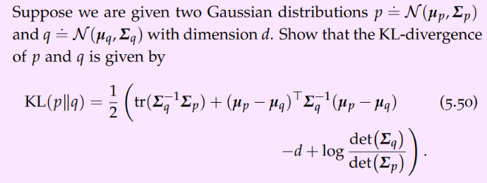
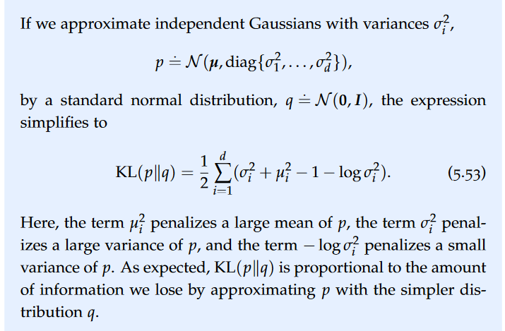
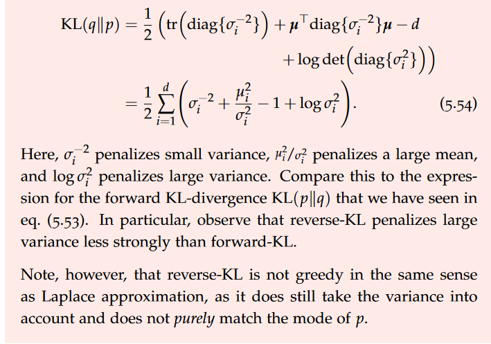
KL-divergence of Gaussians

Alt text

Alt text

Alt text

Evidence Lower Bound

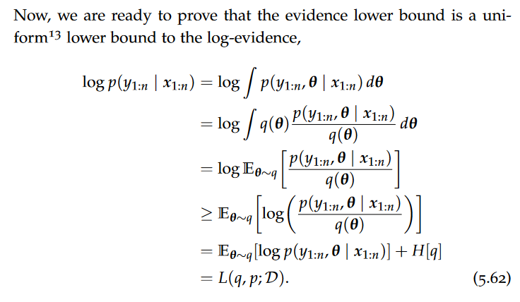
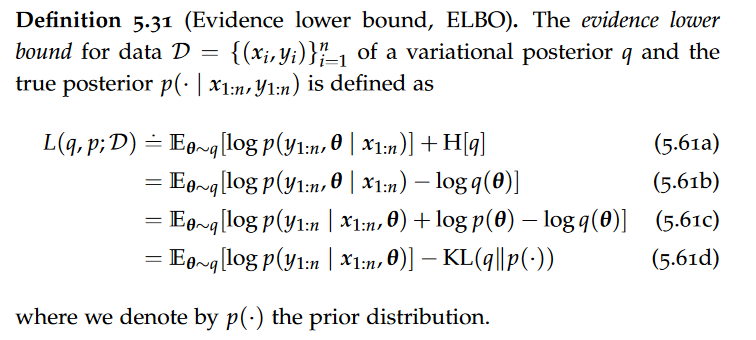
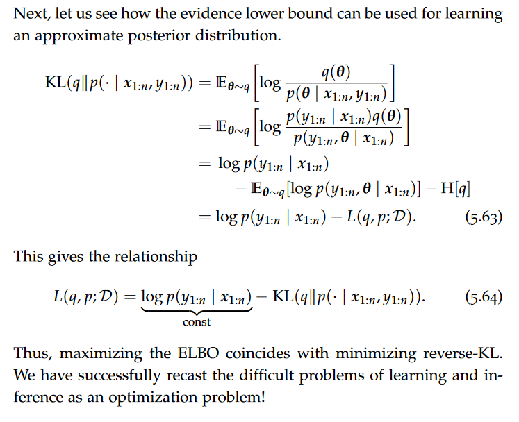
The Evidence Lower Bound is a quantity maximization of which is equivalent to minimizing the KL-divergence. As its name suggests, the evidence lower bound is a (uniform) lower bound to the log-evidence $log p(y{1:n}|x{1:n})$.
Alt text

Alt text

Note that this inequality lower bounds the logarithm of an integral by an expectation of a logarithm over some variational distribution q. Hence, the ELBO is a family of lower bounds — one for each variational distribution. Such inequalities are called variational inequalities.

Alt text

Gradient of Evidence Lower Bound

Alt text
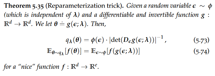
Obtaining the gradient of the evidence lower bound is more difficult. This is because the expectation integrates over the measure $q_\lambda$, which depends on the variational parameters $\lambda$. Thus, we cannot move the gradient operator inside the expectation.

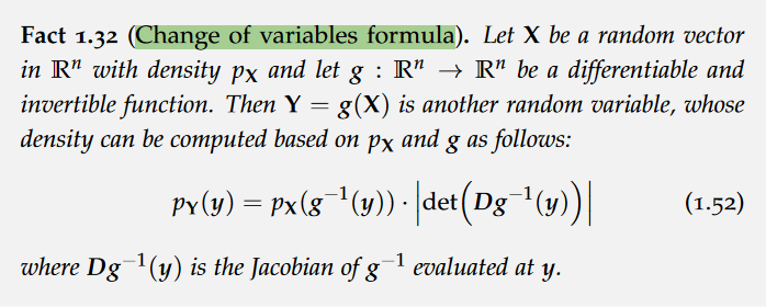
There are two main techniques which are used to rewrite the gradient in such a way that Monte Carlo sampling becomes possible. The first is to use score gradients. The second is the so-called reparameterization trick.

reparameterization trick

Alt text
Alt text

Alt text

The procedure of approximating the true posterior using a variational posterior by maximizing the evidence lower bound using stochastic optimization is also called black box stochastic variational inference. The only requirement is that we can obtain unbiased gradient estimates from the evidence lower bound (and the likelihood).