metrics

BLEU (Bilingual Evaluation Understudy)

BLEU computes a score based on the n-gram overlap between the generated text and the reference text, as well as the brevity penalty to handle cases where the generated text is too short. The score ranges from 0 to 1, where 1 indicates a perfect match with the reference translations.

ROUGE (Recall-Oriented Understudy for Gisting Evaluation)

ROUGE score measures the similarity between the machine-generated summary and the reference summaries using overlapping n-grams, word sequences that appear in both the machine-generated summary and the reference summaries. ROUGE score ranges from 0 to 1, with higher values indicating better summary quality.

ROUGE scores are branched into ROUGE-N,ROUGE-L, and ROUGE-S.
ROUGE-N measures the overlap of n-grams (contiguous sequences of n words) between the candidate text and the reference text. It computes the precision, recall, and F1-score based on the n-gram overlap.
ROUGE-L measures the longest common subsequence (LCS) between the candidate text and the reference text. It computes the precision, recall, and F1-score based on the length of the LCS.
ROUGE-S measures the skip-bigram (bi-gram with at most one intervening word) overlap between the candidate text and the reference text. It computes the precision, recall, and F1-score based on the skip-bigram overlap.

references

https://medium.com/@sthanikamsanthosh1994/understanding-bleu-and-rouge-score-for-nlp-evaluation-1ab334ecadcb

fundamentals

probability

sample space, event space, σ-algebra and probability space

A probability space is a mathematical construct that consists of three elements: the sample space (S), the event space (E), and a probability measure (P). Additionally, a sigma-algebra (σ-algebra) is associated with the event space.

The sample space is the set of all possible outcomes of an experiment.The event space is a collection of subsets of the sample space.
A sigma-algebra is a collection of subsets of the sample space. It includes the sample space, is closed under complementation, and is closed under countable unions. The probability measure is a function that assigns probabilities to events.

probability mass function (PMF) and cumulative distribution function (CDF),probability density function (PDF)

The Probability Mass Function (PMF) is a function that gives the probability that a discrete random variable is exactly equal to a certain value. The Cumulative Distribution Function (CDF) of a random variable gives the probability that
X takes on a value less than or equal to x.
The Probability Density Function (PDF) is applicable to continuous random variables.The total area under the PDF curve is equal to 1.

Continuous Distributions

normal distribution(Gaussian):The Gaussian CDF cannot be expressed in closed-form. Note that the mean of a Gaussian distribution coincides with the maximizer of its PDF, also called mode of a distribution.

Joint Probability, Conditional Probability, Sum rule, Product rule(chain rule),the law of total probability

Joint probability refers to the probability of the occurrence of two or more events simultaneously. Conditional probability is the probability of one event occurring given that another event has already occurred. The sum rule, or addition rule, gives the probability of the union of two events. The product rule, also known as the chain rule, provides a way to express the joint probability of multiple events. The law of total probability is a way to express the probability of an event B by considering all possible ways in which
B can occur.

independence, conditional independence

Conditional independence does not necessarily imply unconditional independence, and vice versa.

Directed Graphical Models(Bayesian networks)

Directed graphical models (also called Bayesian networks) are often used to visually denote the (conditional) independence relationships of a large number of random variables.

Expectation, Covariance and Variance, Standard deviation,Law of total variance

Change of variables formula

Probabilistic inference

Bayes’ rule,Conjugate Priors

gaussian,Guassian random vector

Any affine transformation of a Gaussian random vector is a Gaussian random vector.

Supervised Learning and Point Estimates

Maximum Likelihood Estimation,Maximum a Posteriori Estimation,

The MLE and MAP estimate can be seen as a naïve approximation of probabilistic inference, represented by a point density which “collapses” all probability mass at the mode of the posterior distribution.

exercise

affine transformation,Jacobian matrix,

PML

linear regression

linear regression(MLE), ridge regression(MAP)

ridge,lasso

least absolute shrinkage and selection operator (lasso): Laplace prior, L1 regularization.
Ridge: Gaussian prior, L2 regularization.

The primary difference lies in the penalty terms: L1 regularization uses the sum of absolute values, and L2 regularization uses the sum of squared values.
L1 regularization tends to result in exact zeros, leading to sparse solutions, whereas L2 regularization generally leads to smaller, non-zero coefficients.

Bayesian linear regression (BLR)

Aleatoric and Epistemic Uncertainty

epistemic uncertainty: corresponds to the uncertainty about our model due to the lack of data. aleatoric uncertainty: “irreducible noise”, cannot be explained by the inputs and any model from the model class.

equation under the law of total variance.

kernel

Filtering

The process of keeping track of the state using noisy observations is also known as Bayesian filtering or recursive Bayesian estimation.

Kalman filter

A Kalman filter is simply a Bayes filter using a Gaussian distribution over the states and conditional linear Gaussians to describe the evolution of states and observations.

Gaussian Process

A Gaussian process is an infinite set of random variables such that any finite number of them are jointly Gaussian.

kernel function, feature space, RKHS,Stationarity and isotropy

A Gaussian process with a linear kernel is equivalent to Bayesian linear regression.

For ν = 1/2, the Matérn kernel is equivalent to the Laplace kernel. For ν → ∞, the Matérn kernel is equivalent to the Gaussian kernel.

Note that stationarity is a necessary condition for isotropy. In other words, isotropy implies stationarity.

skip 4.3.4

model selection

Maximizing the Marginal Likelihood

Marginal likelihood maximization is an empirical Bayes method. Often it is simply referred to as empirical Bayes.
this approach typically avoids overfitting even though we do not use a separate training and validation set. maximizing the marginal likelihood naturally encourages trading between a large likelihood and a large prior.

Approximations

random Fourier features,Bochner’s theorem,Uniform convergence of Fourier features

inducing points method,subset of regressors (SoR) approximation,fully independent training conditional (FITC) approximation

Variational Inference

Laplace Approximation,Bayesian Logistic Regression,

The Laplace approximation matches the shape of the true posterior around its mode but may not represent it accurately elsewhere — often leading to extremely overconfident predictions.

Variational family,mean-field distribution

Information Theory,Surprise,entropy,Jensen’s Inequality,Cross-entropy,KL-divergence,Forward and Reverse KL-divergence

The uniform distribution has the maximum entropy among all discrete distributions supported on {1, . . . , n}.

In words, KL(p∥q) measures the additional expected surprise when observing samples from p that is due to assuming the (wrong) distribution q.

It can be seen that the reverse KL-divergence tends to greedily select the mode and underestimating the variance which, in this case, leads to an overconfident prediction. The forward KL-divergence, in contrast, is more conservative.

Note, however, that reverse-KL is not greedy in the same sense as Laplace approximation, as it does still take the variance into account and does not purely match the mode of p.

Minimizing Forward-KL as Maximum Likelihood Estimation,Minimizing Forward-KL as Moment Matching

First, we observe that minimizing the forward KL-divergence is equivalent to maximum likelihood estimation on an infinitely large sample size.

A Gaussian qλ minimizing KL(p∥qλ) has the same first and second moment as p.

Evidence Lower Bound,Gaussian VI vs Laplace approximation, Gradient of Evidence Lower Bound(score gradients and Reparameterization trick)

maximizing the ELBO coincides with minimizing reverse-KL.

maximizing the ELBO selects a variational distribution q that is close to the prior distribution p(·) while also maximizing the average likelihood of the data p(y1:n | x1:n, θ) for θ ∼ q.

Note that for a noninformative prior p(·) ∝ 1, maximizing the ELBO is equivalent to maximum likelihood estimation.

skip 5.5.2

Markov Chain Monte Carlo Methods

The key idea of Markov chain Monte Carlo methods is to construct a Markov chain, which is efficient to simulate and has the stationary distribution p.

Markov Chains(Stationarity,convergence), Markov property,time-homogeneous Markov chains

Intuitively, the Markov property states that future behavior is independent of past states given the present state.

Stationary distribution,aperiodic,Ergodicity,Fundamental theorem of ergodic Markov chains

After entering a stationary distribution π, a Markov chain will always remain in the stationary distribution.

It can be shown that there exists a unique stationary distribution π if the Markov chain is irreducible, that is, if every state is reachable from every other state with a positive probability when the Markov chain is run for enough steps.

Even if a Markov chain has a unique stationary distribution, it must not converge to it.

In words, a Markov chain is aperiodic iff for every state x, the transition graph has a closed path from x to x with length k for all k ∈ N greater than some k0 ∈ N.

A Markov chain is ergodic iff there exists a t ∈ N0 such that for any x, x′ ∈ S we have p(t)(x′ | x) > 0.

A commonly used strategy to ensure that a Markov chain is ergodic is to add “self-loops” to every vertex in the transition graph.

An ergodic Markov chain has a unique stationary distribution π (with full support) irrespectively of the initial distribution q0. This naturally suggests constructing an ergodic Markov chain such that its stationary distribution coincides with the posterior distribution. If we then sample “sufficiently long”, Xt is drawn from a distribution that is “very close” to the posterior distribution.

How quickly does a Markov chain converge?(Total variation distance and Mixing time)

Detailed Balance Equation,Ergodic Theorem

A Markov chain that satisfies the detailed balance equation with respect to π is called reversible with respect to π.

Ergodic Theorem is a way to generalize the (strong) law of large numbers to Markov chains.

Elementary Sampling Methods,Metropolis-Hastings Algorithm,Metropolis-Hastings theorem, Gibbs Sampling

A popular example of a Metropolis-Hastings algorithm is Gibbs sampling.

Sampling as Optimization,Gibbs distribution,Langevin Dynamics,Metropolis adjusted Langevin algorithm (MALA) or Langevin Monte Carlo (LMC),unadjusted Langevin algorithm (ULA), Stochastic Gradient Langevin Dynamics, Hamiltonian Monte Carlo

A useful property is that Gibbs distributions always have full support. Observe that the posterior distribution can always be interpreted as a Gibbs distribution as long as prior and likelihood have full support.

Langevin dynamics adapts the Gaussian proposals of the Metropolis-Hastings algorithm to search the state space in an “informed” direction. The simple idea is to bias the sampling towards states with lower energy, thereby making it more likely that a proposal is accepted. A natural idea is to shift the proposal distribution perpendicularly to the gradient of the energy function. The resulting variant of Metropolis-Hastings is known as the Metropolis adjusted Langevin algorithm (MALA) or Langevin Monte Carlo (LMC).

The HMC algorithm is an instance of Metropolis-Hastings which uses momentum to propose distant points that conserve energy, with high acceptance probability.

path

target: show that the stationary distribution of a Markov chain coincides with the posterior distribution.
base: Detailed Balance Equation which shows that A Markov chain that satisfies the detailed balance equation with respect to π is called reversible with respect to π and if the Markov chain is reversible with respect to π then π is a stationary distribution. With posterior distribution p(x) = 1/Z q(x), substitute the posterior for π in the detailed balance equation, we can remove z, so we do not need to know the true posterior p to check that the stationary distribution of our Markov chain coincides with p, it suffices to know the finite measure q. However, until now, this does not allow us to estimate expectations over the posterior distribution. Note that although constructing such a Markov chain allows us to obtain samples from the posterior distribution, they are not independent. Thus, the law of large numbers and Hoeffding’s inequality do not apply, but there is a way to generalize the (strong) law of large numbers to Markov chains, which is Ergodic theorem.

Next we need to consider how to construct Markov chain with the goal of approximating samples from the posterior distribution p. One way is Metropolis-Hastings Algorithm, in which we are given a proposal distribution and we use the acceptance distribution to decide whether to follow the proposal. Another way is Gibbs sampling.

MCMC techniques can be generalized to
continuous random variables / vectors. Observe that the posterior distribution can always be interpreted as a Gibbs distribution as long as prior and likelihood have full support.

Langevin dynamics adapts the Gaussian proposals of the Metropolis-Hastings algorithm to search the state space in an “informed” direction. The simple idea is to bias the sampling towards states with lower energy, thereby making it more likely that a proposal is accepted. A natural idea is to shift the proposal distribution perpendicularly to the gradient of the energy function. The resulting variant of Metropolis-Hastings is known as the Metropolis adjusted Langevin algorithm (MALA) or Langevin Monte Carlo (LMC).

skip 6.3.5

BDL

Artificial Neural Networks,Activation Functions,

Non-linear activation functions allow the network to represent arbitrary functions. This is known as the universal approximation theorem.

Bayesian Neural Networks, Heteroscedastic Noise, Variational Inference,Markov Chain Monte Carlo, SWA,SWAG,Dropout and Dropconnect, Probabilistic Ensembles

Intuitively, variational inference in Bayesian neural networks can be interpreted as averaging the predictions of multiple neural networks drawn according to the variational posterior qλ.

Calibration,expected calibration error (ECE), maximum calibration error (MCE), Histogram binning, Isotonic regression, Platt scaling, Temperature scaling

We say that a model is wellcalibrated if its confidence coincides with its accuracy across many predictions. Compare within each bin, how often the model thought the inputs belonged to the class (confidence) with how often the inputs actually belonged to the class (frequency).

Sequential Decision-Making

Active Learning

Conditional Entropy,Joint entropy

A very intuitive property of entropy is its monotonicity: when conditioning on additional observations the entropy can never increase.

Mutual Information(information gain), the law of total expectation, data processing inequality, interaction information(Synergy and Redundancy), Submodularity of Mutual Information, Marginal gain, Submodularity, monotone,

data processing inequality: which says that processing cannot increase the information contained in a signal.

F is submodular iff “adding” x to the smaller set A yields more marginal gain than adding x to the larger set B.

I is monotone submodular.

Maximizing Mutual Information, Greedy submodular function maximization, Uncertainty Sampling, Marginal gain of maximizing mutual information,Bayesian active learning by disagreement (BALD)

skip proof of Theorem 8.15

Therefore, if f is modeled by a Gaussian and we assume homoscedastic noise, greedily maximizing mutual information corresponds to simply picking the point x with the largest variance. This algorithm is also called uncertainty sampling.

Experimental Design, Entropy Search

skip

Bayesian Optimization

Exploration-Exploitation Dilemma,Online Learning and Bandits, Multi-Armed Bandits, Regret, sublinear regret, Cesàro mean

Bayesian optimization can be interpreted as a variant of the MAB problem where there can be a potentially infinite number of actions (arms), but their rewards are correlated (because of the smoothness of the Gaussian process prior).

Acquisition Functions, Upper Confidence Bound, Bayesian confidence intervals, Regret of GP-UCB, Information gain of common kernels, Frequentist confidence intervals, probability of improvement, expected improvement (EI), Thompson Sampling, probability matching, Information-Directed Sampling

skip Information-Directed Sampling

Markov Decision Processes

Planning deals with the problem of deciding which action an agent should play in a (stochastic) environment. A key formalism for probabilistic planning in known environments are so-called Markov decision processes.

Policy,discounted payoff,state value function,state-action value function (also called Q-function)

A policy is a function that maps each state x ∈ X to a probability distribution over the actions.

Bellman Expectation Equation

Policy Evaluation, Fixed-point Iteration, contraction,Banach fixed-point theorem

Policy Optimization, Greedy Policies, Bellman Optimality Equation, Bellman’s theorem, Policy Iteration, Value Iteration,

In particular, if for every state there is a unique action that maximizes the state-action value function, the policy π⋆ is deterministic and unique.

Intuitively, the Bellman optimality equations express that the value of a state under an optimal policy must equal the expected return for the best action from that state.

Value iteration converges to an ε-optimal solution in a polynomial number of iterations. Unlike policy iteration, value iteration does not converge to an exact solution in general.

Partial Observability,

Whereas MDPs are controlled Markov chains, POMDPs are controlled hidden Markov models.

Tabular Reinforcement Learning

Trajectories, episodic setting, continuous setting, On-policy and Off-policy Methods,

on-policy methods are used when the agent has control over its own actions, in other words, the agent can freely choose to follow any policy. off-policy methods can be used even when the agent cannot freely choose its actions.

Model-based Approaches, Balancing Exploration and Exploitation, ε-greedy, Softmax Exploration(Boltzmann exploration), Rmax algorithm

skip Remark 11.3: Asymptotic convergence

Note that ε-greedy is GLIE with probability 1 if the sequence (εt)t∈N0 satisfies the RM-conditions (A.56), e.g., if εt = 1/t.

A significant benefit to model-based reinforcement learning is that it is inherently off-policy. That is, any trajectory regardless of the policy used to obtain it can be used to improve the model of the underlying Markov decision process. In the model-free setting, this not necessarily true.

Model-free Approaches, On-policy Value Estimation, bootstrapping, temporal-difference learning, SARSA, Off-policy Value Estimation, Q-learning, optimistic Q-learning

Model-free Reinforcement Learning

Value Function Approximation, DQN, experience replay, maximization bias, Double DQN

Policy Approximation(policy gradient methods), policy value function, Policy Gradient, Score gradient estimator, Score gradients with baselines, Downstream returns, REINFORCE algorithm

The main advantage of policy gradient methods such as REINFORCE is that they can be used in continuous action spaces. However, REINFORCE is not guaranteed to find an optimal policy. Even when operating in very small domains, REINFORCE can get stuck in local optima.

On-policy Actor-Critics,Advantage Function, Policy Gradient Theorem, Actor-Critic(Q actor-critic,Online actor-critic), advantage actor-critic, bias-variance tradeoff, trust-region policy optimization (TRPO), Proximal policy optimization (PPO)

One approach in the online setting (i.e., non-episodic setting), is to simply use SARSA for learning the critic. To learn the actor, we use stochastic gradient descent with gradients obtained using single samples.

Model-based Reinforcement Learning

Planning over Finite Horizons, receding horizon control (RHC), model predictive control (MPC), Random shooting methods

cheat sheet

from book

conditional distribution for gaussian;
Gaussian process posterior;
the predictive posterior at the test point;
common kernels;
the Hessian of the logistic loss;
Surprise,entropy,Jensen’s Inequality,Cross-entropy,KL-divergence,
ELBO,
the law of large numbers and Hoeffding’s inequality,
Hoeffding bound,

from exercise

Woodbury push-through identity;
Solution to problem 3.6;

data cubes

slides

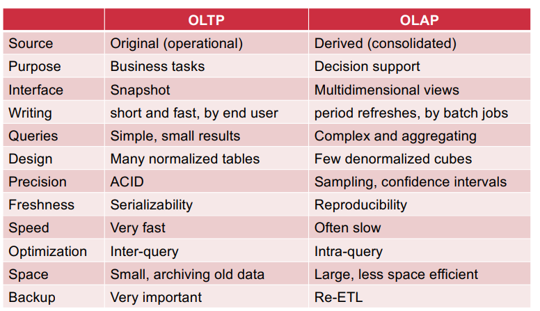
OLTP VS OLAP:

record keeping vs decision support
read-intensive vs write-intensive
detailed individual records vs summarized data
Lots of transactions on small portions of data vs Large portions
of the data.
fully interactive vs slow interactive.

ETL: Extract Transform Load

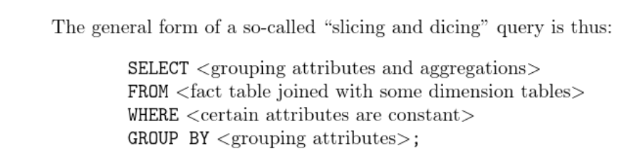
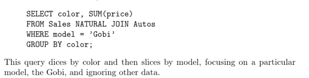
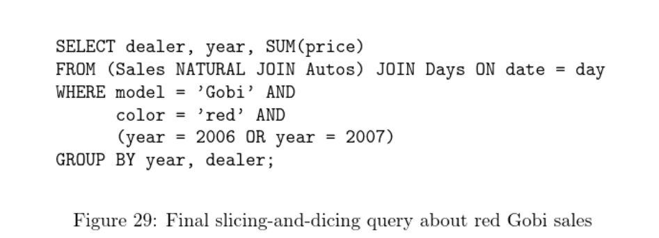
slicing and dicing,Pivoting

Slicing involves selecting a specific “slice” or subset of the data cube by fixing one or more dimensions at a particular value. Dicing involves creating a subcube by selecting specific values for two or more dimensions. It’s like slicing, but you are selecting a rectangular subset of the cube, cutting through more than one dimension. Pivoting is another operation often used alongside slicing and dicing. It involves rotating the data cube to view it from a different perspective by swapping the positions of dimensions.

Aggregation and roll-up

These operations allow users to summarize and view data at different levels of granularity within a multidimensional dataset. Roll-up is a specific form of aggregation that involves moving from a lower level of detail to a higher level by collapsing one or more dimensions(moving up the hierarchy from a finer level of granularity (monthly) to a coarser level (quarterly)).

Two flavors of OLAP: ROLAP and MOLAP

ROLAP (Relational Online Analytical Processing) and MOLAP (Multidimensional Online Analytical Processing) are two different approaches to organizing and processing data in the context of Online Analytical Processing (OLAP) systems. In summary, the main difference between ROLAP and MOLAP lies in how they store and organize data. ROLAP uses relational databases to store multidimensional data in tables, while MOLAP uses specialized databases with a cube structure optimized for efficient multidimensional analysis.

fact table and Satellite table

Fact tables are surrounded by dimension tables in a star schema. They usually have foreign key relationships with dimension tables, linking to various dimensions that provide context to the measures. Satellite tables are used to store additional details about dimension members that are not part of the core structure of the dimension table. Satellite tables typically have a foreign key relationship with the main dimension table, linking to the primary key of the dimension. They can be joined to the main dimension table to enrich the analysis with additional context.

star schema and snow-flake schema

In a star schema, there is a central fact table surrounded by dimension tables. The fact table contains quantitative data (measures), and the dimension tables store descriptive data related to the measures. A snowflake schema is an extension of the star schema, where dimension tables are normalized into multiple related tables. This normalization leads to a structure resembling a snowflake when visualized, as opposed to the star-like structure of a star schema.

SQL querying tables and MDX querying Cubes

MDX stands for Multi-Dimensional
eXpressions.

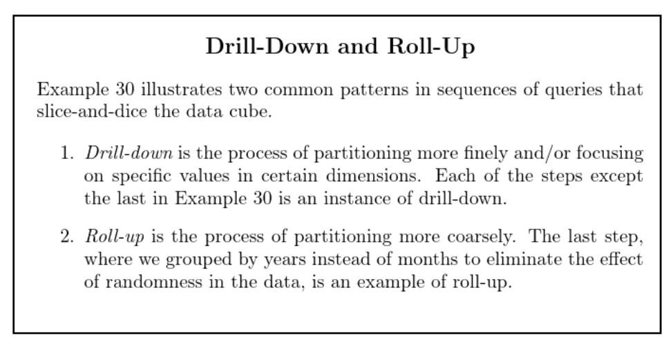
“Roll-up” and “drill down”

Roll-up involves summarizing data at a higher level of aggregation or moving from a lower level of detail to a higher level. It’s a way of viewing data at a coarser level in the hierarchy. Drill down is the opposite of roll-up. It involves accessing more detailed information or moving from a higher level of aggregation to a lower, more detailed level.

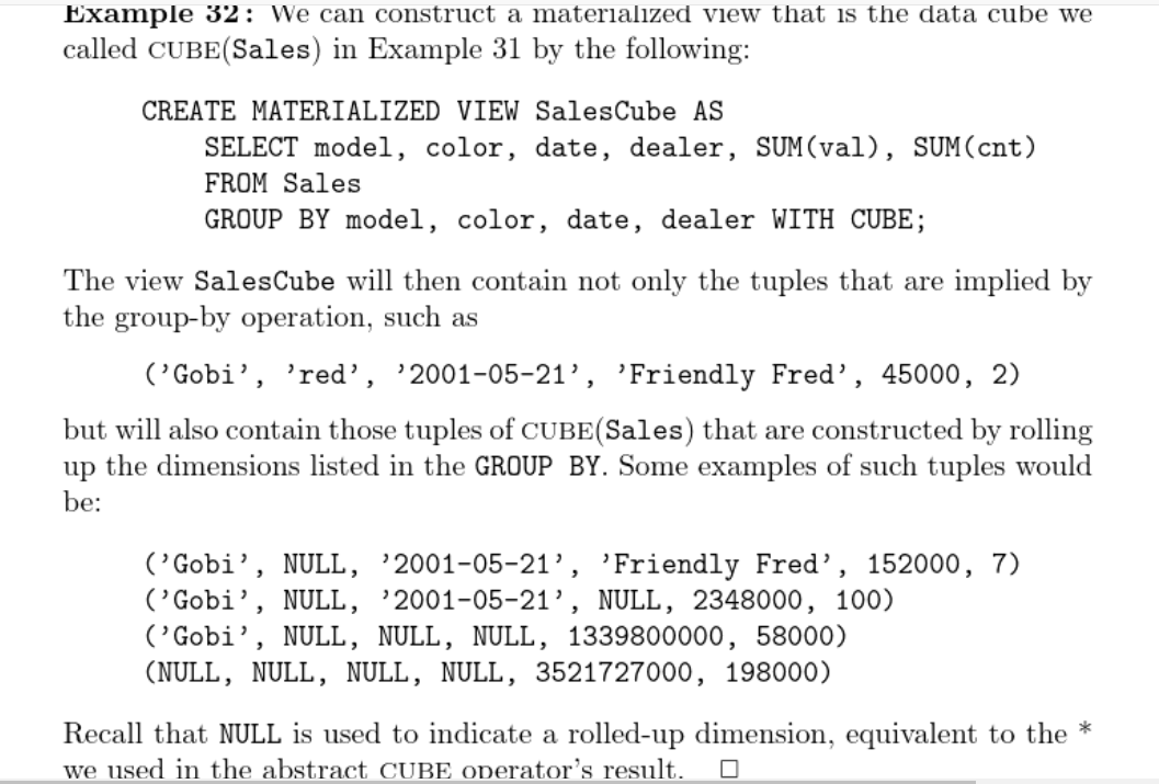
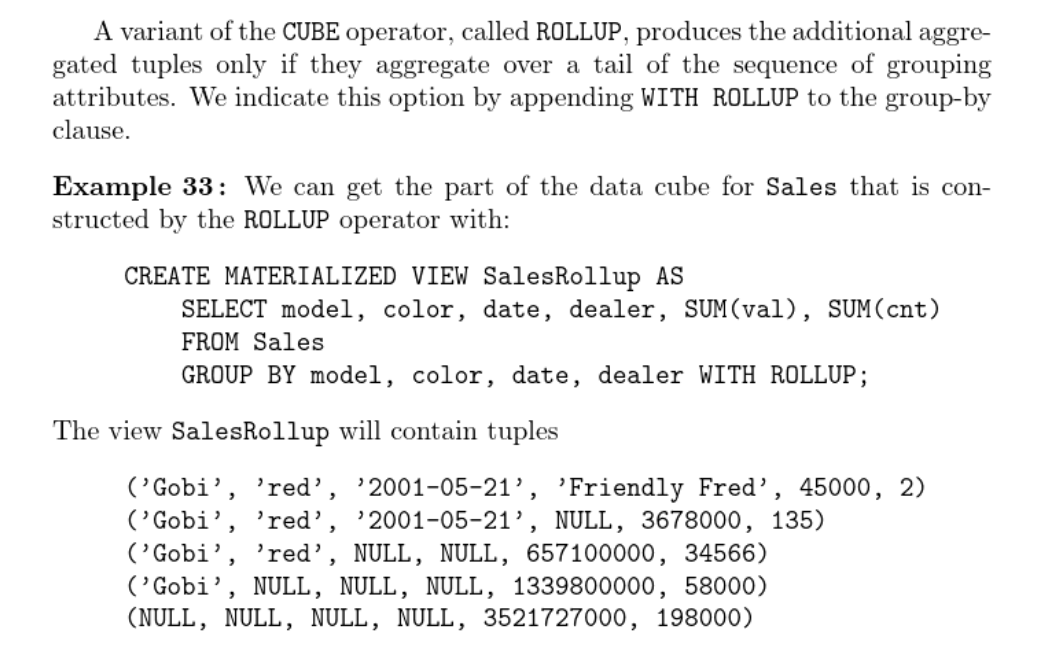
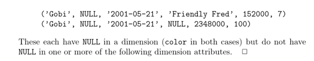
GROUPING SETS, CUBE, ROLLUP

GROUPING SETS is a SQL feature that allows you to specify multiple grouping sets within a single query. The CUBE operation is an extension of GROUP BY that generates all possible combinations of grouped elements. ROLLUP is another extension of GROUP BY that generates subtotals and grand totals for a specified set of columns. It creates a hierarchy of grouping levels, calculating subtotals as it rolls up the hierarchy. Note that the column order in rollup is important.

book

exercise

concepts of fact tables;
pivot table;
SQL query with grouping set, cube…

Graph Databases

sildes

Index-free adjacency

With index-free adjacency, graph databases are designed in such a way that relationships between nodes are directly accessible without the need for an index structure. Instead of traversing indexes to find related nodes, the relationships are stored alongside the nodes, allowing for faster and more efficient traversal.Each node maintains direct pointers or references to its neighboring nodes, making it possible to navigate from one node to another without the need for an explicit index lookup. This design principle is particularly beneficial for scenarios where traversing relationships in a graph is a common and performance-critical operation.

Property Graph and Triple stores (RDF)

Labeled property graphs: ingredients: Nodes, Edges,Properties,Labels.
A property graph is a graph data model that consists of nodes, edges, and properties.RDF is a standard for representing data about resources in the form of subject-predicate-object triples.

Cypher

Cypher is a query language commonly used with property graph databases like Neo4j.

SPARQL

SPARQL is a query language commonly used with RDF triple stores.

Neo4j

Data replication;
sharding:neo4j fabric;
Caching and pages;

RDF

IRI (=URI for all practical purposes);

RDF formats:RDF/XML;Turtle;JSON-LD;RDFa;N-Triples.

book

Labeled property graph model vs. triple stores

labeled property graphs enhance mathematical graphs with extra ingredients: properties, and labels.
Labels are some sort of “tags”, in the form of a string, that can be attached to a node or an edge.
Each node and each edge can be associated with a map from strings to values, which represents its properties.

Triple stores are a different and simpler model. It views the graph as nodes and edges that all have labels, but without any properties.
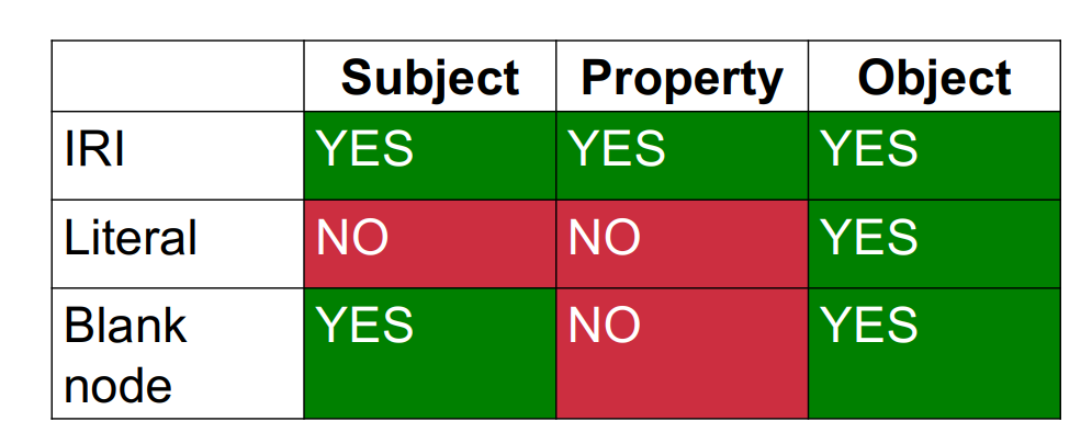
The graph is then represented as a list of edges, where each edge is a triple with the label of the origin node (called the subject), the label of the edge (called the property), and the label of the destination node (called the object).

Labels can be:URIs,Literals, that is, atomic values,Literals are only allowed as objects. Absent, in which case the node is called a blank node. Blank nodes are only allowed as subjects or objects, but not as properties.

cypher

Other graph databases have other means of querying data. Many, including Neo4j, support the RDF query language SPARQL and the imperative, path-based query language Gremlin.

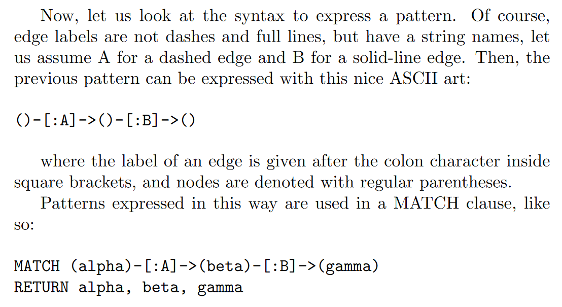
Cypher enables a user (or an application acting on behalf of a user) to ask the database to find data that matches a specific pattern. Colloquially, we ask the database to “find things like this.” And the way we describe what “things like this” look like is to draw them, using ASCII art.

The MATCH clause is at the heart of most Cypher queries.

native graph processing

To understand why native graph processing is so much more efficient than graphs based on heavy indexing, consider the following. Depending on the implementation, index lookups could be O(log n) in algorithmic complexity versus O(1) for looking up immediate relationships. To traverse a network of m steps, the cost of the indexed approach, at O(m log n), dwarfs the cost of O(m) for an implementation that uses index-free adjacency.

With index-free adjacency, bidirectional joins are effectively precomputed and stored in the database as relationships

stores

Neo4j stores graph data in a number of different store files. Each store file contains the data for a specific part of the graph (e.g., there are separate stores for nodes, relationships, labels, and properties). Like most of the Neo4j store files, the node store is a fixed-size record store, where each record is nine bytes in length. Fixed-size records enable fast lookups for nodes in the store file.

CYPHER,Traverser API and Core API

Neo4j’s Core API is an imperative Java API that exposes the graph primitives of nodes, relationships, properties, and labels to the user. When used for reads, the API is lazily evaluated, meaning that relationships are only traversed as and when the calling code demands the next node.

The Traversal Framework is a declarative Java API. It enables the user to specify a set of constraints that limit the parts of the graph the traversal is allowed to visit.

Cypher can be more tolerant of structural changes—things such as variable-length paths help mitigate variation and change.

however, the Traversal Framework tends to perform marginally less well than a well-written Core API query.

Choosing between the Core API and the Traversal Framework is a matter of deciding whether the higher abstraction/lower coupling of the Traversal Framework is sufficient, or whether the close-to-the-metal/higher coupling of the Core API is in fact necessary for implementing an algorithm correctly and in accordance with our performance requirements.

exercise

Querying trees

slides

JSONiq

Data independence with
heterogeneous, denormalized data.
JSONiq Data Model (JDM): Sequences of Items;

Declarative languages,Functional languages and Set-based languages

Declarative languages focus on describing what the program should accomplish, rather than specifying how to achieve it. Functional languages treat computation as the evaluation of mathematical functions and avoid changing state or mutable data.Haskell, Lisp, and Erlang are functional programming languages.
Parts of JavaScript and Python support functional programming paradigms. Set-based languages are a subset of declarative languages that focus on manipulating sets of data.
It’s worth noting that languages can often belong to more than one category. For example, SQL is both declarative and set-based, and functional programming concepts can be integrated into languages that are not purely functional.

FLWOR clauses

query,Abstract Syntax Tree, Expression Tree, Iterator Tree

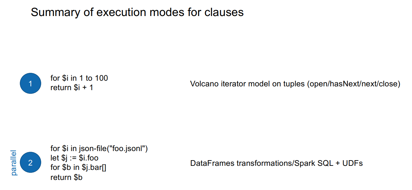
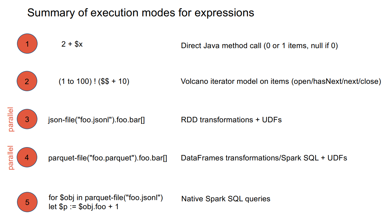
Materialized execution,Streamed execution,Parallel execution

Materialized execution takes lots of space. Streamed execution takes lots of time.
Parallel execution can take lots of machines.
Execution modes determined statically for every expression and clause.

Rumble

Traditional RDBMS/warehouses vs. data lakes

book

exercise

Document Stores

slides

JSON and XML

SQL and NoSQL:

NoSQL: validation after the data was populated.

CRUD

Create,Read,Update,Delete

MongoDB

projecting away: not selecting a field.

hash indices,Tree indices (B+-tree),compund index

Limitations of hash indices:
No support for range queries,Hash function not perfect in real life, Space requirements for collision avoidance.
B+-tree: All leaves at same depth, All non-leaf nodes have between 3 and 5 children,But it’s fine if the root has less.

book

exercise

Performance at Large Scales

slides

sources of bottleneck

Memory, CPU, Disk I/O, Network I/O.
Sweet Spot for MapReduce and Spark: Disk I/O.

Latency, Throughput,Response time

Latency: When do I start receiving data.
Throughput:”How fast can we transmit data.
Response time=Latency + Transfer.

speedup,Amdahl’s law,Gustafson’s law

speedup = latency(old)/latency(new).
Gustafson’s law:Constant computing power.
Amdahl’s law: Constant problem size.

Scaling out,Scaling up

tail latency, SLA

book

exercise

Massive Parallel Processing I(MapReduce)

slides

combine and reduce

map task and reduce task, map slot and reduce slot, map phase amd reduce phase

no combine task and combine slot.
map slot = sequential map task; map task = sequential split map;

split(mapreduce) and block(HDFS)

1 split = 1 map task
split(mapreduce)!= block(HDFS)

book

mapreduce model

In MapReduce, the input data, intermediate data, and output data are all made of a large collection of key-value pairs (with the keys not necessarily unique, and not necessarily sorted by key).

MapReduce architecture

In the original version of MapReduce, the main node is called JobTracker, and the worker nodes are called TaskTrackers.
In fact, the JobTracker typically runs on the same machine as the NameNode (and HMaster) and the TaskTrackers on the same machines as the DataNodes (and RegionServers). This is called “bring the query to the data.”

Note that shuffling can start before the map phase is over, but the reduce phase can only start after the map phase is over.

combine

Combining happens during the map phase.
In fact, in most of the cases, the combine function will be identical to the reduce function, which is generally possible if the intermediate key-value pairs have the same type as the output key-value pairs, and the reduce function is both associative and commutative.

MapReduce programming API

In Java, the user needs to define a so-called Mapper class that contains the map function, and a Reducer class that contains the reduce function.
A map function takes in particular a key and a value. Note that it outputs key-value pairs via the call of the write method on the context, rather than with a return statement.
A reduce function takes in particular a key and a list of values.

function,task,slot,phase

A map function is a mathematical, or programmed, function that takes one input key-value pair and returns zero, one or more intermediate key-value pairs.
Then, a map task is an assignment (or “homework”, or “TODO”) that consists in a (sequential) series of calls of the map function on a subset of the input.

There is no such thing as a combine task. Calls of the combine function are not planned as a task, but is called ad-hoc during flushing and compaction.

The map tasks are processed thanks to compute and memory resources (CPU and RAM). These resources are called map slots. One map slot corresponds to one CPU core and some allocated memory. Each map slot then processes one map task at a time, sequentially.

The map phase thus consists of several map slots processing map tasks in parallel.

short-circuiting(split and block)

This is because the DataNode process of HDFS and the TaskTracker process of MapReduce are on the same machine. Thus, getting a replica of the block containing the data necessary to the processing of the task is as simple as a local read. This is called short-circuiting.
split(logical level)!=HDFS block(physical level).

exercise

Resource management

book

YARN

YARN means Yet Another Resource manager. It was introduced as an additional layer that specifically handles the management of CPU and memory resources in the cluster.
YARN, unsurprisingly, is based on a centralized architecture in which the coordinator node is called the ResourceManager, and the worker nodes are called NodeManagers. NodeManagers furthermore provide slots (equipped with exclusively allocated CPU and memory) known as containers.

YARN provides generic support for allocating resources to any application and is application-agnostic. When the user launches a new application, the ResourceManager assigns one of the container to act as the ApplicationMaster which will take care of running the application.

Version 2 of MapReduce works on top of YARN by leaving the job lifecycle management to an ApplicationMaster.
It is important to understand that, unlike the JobTracker, the ResourceManager does not monitor tasks, and will not restart slots upon failure. This job is left to the ApplicationMasters.

Scheduling strategies

FIFO scheduling,Capacity scheduling,Fair scheduling

Dominant Resource Fairness algorithm.

The two (or more) dimensions are projected again to a single dimension by looking at the dominant resource for each user.

Massive Parallel Processing II (Spark)

slides

YARN

ResourceManager + NodeManager; ResourceManager allocates one NodeManager as application master. Application Master communicates with containers. ResourceManager
Does not monitor tasks and Does not restart upon failure. Fault tolerance is on the application master.

spark

Full-DAG query processing.distributed acyclic graph (DAG)
RDD: Resilient Distributed Dataset.

RDD

lazy evaluation:Lazy evaluation means that the execution of transformations on RDDs is deferred until an action is triggered. Instead of immediately executing the transformations, Spark keeps track of the sequence of transformations in the form of a logical execution plan. The actual computation is only performed when an action is called.

A narrow dependency (also known as a narrow transformation) occurs when each partition of the parent RDD contributes to at most one partition of the child RDD. In other words, the number of partitions remains the same before and after the transformation, and each partition of the child RDD depends on a one-to-one relationship with partitions of the parent RDD.

A wide dependency (also known as a wide transformation) occurs when each partition of the parent RDD contributes to multiple partitions of the child RDD. This typically involves operations that require data shuffling or redistribution, such as groupByKey or reduceByKey.

Data Frames

book

Resilient distributed datasets(RDDs)

Resilient means that they remain in memory or on disk on a “best effort” basis, and can be recomputed if need be. Distributed means that, just like the collections of key-value pairs in MapReduce, they are partitioned and spread over multiple machines.
A major difference with MapReduce, though, is that RDDs need not be collections of pairs. Since a key-value pair is a particular example of possible value, RDDs are a generalization of the MapReduce model for input, intermediate input and output.

The RDD lifecycle

Creation,Transformation(Mapping or reducing, in this model, become two very specific cases of transformations.),Action.
transformations:
unary transformations: The filter transformation,The map transformation,The flatMap transformation,The distinct transformation,The sample transformation
Binary transformations: taking the union of two RDDs, take the intersection, take the subtraction.
Pair transformations: Spark has transformations specifically tailored for RDDs of key-value pairs: The key transformation,The values transformation,The reduceByKey transformation, The groupByKey transformation,The sortByKey transformation,The mapValues transformation,The join transformation,The subtractByKey transformation.
Actions: The collect action,The count action,The countByValue action,The take action,The top action,The takeSample action,The reduce action,saveAsTextFile action,saveAsObjectFile action.

Note that Spark, at least in its RDD API, is not aware of any particular format or syntax, i.e., it is up to the user to parse and serialize values to the appropriate text or bytes.

Actions on Pair RDDs: There are actions specifically working on RDDs of key-value pairs:The countByKey action, The lookup action,

Lazy evaluation

It is only with an action that the entire computation pipeline is put into motion, leading to the computation of all the necessary intermediate RDDs all the way down to the final output corresponding to the action.

Physical architecture

There are two kinds of transformations: narrow-dependency transformations and wide-dependency transformations.

Such a chain of narrow-dependency transformations executed efficiently as a single set of tasks is called a stage, which would correspond to what is called a phase in MapReduce.

Optimizations

Pinning RDDs, Pre-partitioning.

DataFrames in Spark

A DataFrame can be seen as a specific kind of RDD: it is an RDD of rows (equivalently: tuples, records) that has relational integrity, domain integrity, but not necessarily (as the name “Row” would otherwise fallaciously suggest) atomic integrity.

Note that Spark automatically infers the schema from discovering the JSON Lines file, which adds a static performance overhead that does not exist for raw RDDs: there is no free lunch.

Unlike the RDD transformation API, there is no guarantee that the execution will happen as written, as the optimizer is free to reorganize the actual computations.

Spark SQL

both GROUP BY and ORDER BY will trigger a shuffle in the system. The SORT BY clause can sort rows within each partition, but not across partitions, i.e., does not induce any shuffling. The DISTRIBUTE BY clause forces a repartition by putting all rows with the same value (for the specified field(s)) into the same new partition.

use both SORT and DISTRIBUTE = the use of another clause, CLUSTER BY.

A word of warning must be given on SORT, DISTRIBUTE and CLUSTER clauses: they are, in fact, a breach of data independence, because they expose partitions.

explode() and lateral view: Lateral views are more powerful and generic than just an explode() because they give more control, and they can also be used to go down several levels of nesting.

book

exercise

Spark’s RDDs are by default recomputed each time you run an action on them. Please note that both persist() and cache() are lazy operations themselves. The caching operation will, in fact, only take place when the first action is called. With successive action calls, the cached RDD will be used.

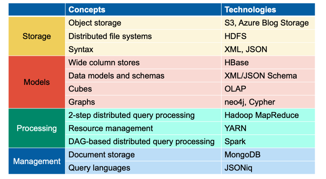
introduction

book

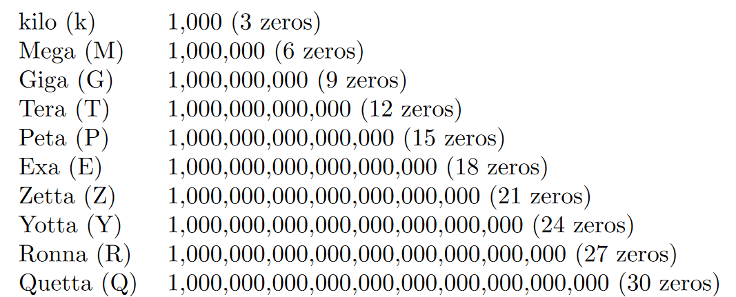
three Vs: Volume, Variety, Velocity.

four more shapes: trees, unstructured, cubes,graphs.
three factors: Capacity,Throughput, Latency.

partial function and function

A function is a strict mapping where every element in the domain is mapped to a unique element in the codomain.
A partial function is a mapping where not every element in the domain necessarily has a defined value in the codomain.
For a table, we need to throw in three additional constraints: relational integrity, domain integrity and atomic integrity.

lessons learned from the past

book

natural join, theta join, and outer join,Semi-outer join

A natural join is a type of join that combines rows from two tables based on columns with the same name and data type. The columns used for the join condition are not explicitly specified; instead, the database system automatically identifies the matching columns. A theta join is a generalization of the natural join, where the join condition is explicitly specified using a comparison operator.

Normal forms

The first normal form was already covered earlier: it is in fact atomic integrity.
The second normal form takes it to the next level: it requires that each column in a record contains information on the entire record. The third normal form additionally forbids functional dependencies on anything else than the primary key.

SQL

SQL is a declarative language, which means that the user specifies what they want, and not how to compute it: it is up to the underlying system to figure out how to best execute the query. It is also a set-based language, in the sense that it manipulates sets of records at a time, rather than single values as is common in other languages. It is also, to some limited extent, a functional language in the sense that it contains expressions that can nest in each other (nested queries).

ACID

There are four main properties (often called ACID):Atomicity,Consistency,Isolation,Durability.

exercise

SQL

1NF,2NF,3NF,BCNF;
intersection;

Storing data

book

CAP

(Atomic) Consistency, Availability, Partition tolerance.

document stores

book

Document stores provide a native database management system for semi-structured data. A document store typically specializes in either JSON or XML data, even though some companies (e.g., MarkLogic) offer support for both. It is important to understand that document stores are optimized for the typical use cases of many records of small to medium sizes. Typically, a collection can have millions or billions of documents, while each single document weighs no more than 16 MB (or a size in a similar magnitude).

MongoDB

In MongoDB, the format is a binary version of JSON called BSON.

The API of MongoDB, like many document stores, is based on the CRUD paradigm. CRUD means Create, Read, Update, Delete.

MongoDB automatically adds to every inserted document a special field called “ id” and associated with a value called an Object ID and with a type of its own.

hash indices and tree indices

Hash indices are used to optimize point queries and more generally query that select on a specific value of a field.

Secondary indices

By default, MongoDB always builds a tree index for the id field. Users can request to build hash and tree indices for more fields. These indices are called secondary indices.

exercise

By default, MongoDB creates the _id index, which is an ascending unique index on the _id field, for all collections when the collection is created. You cannot remove the index on the _id field.

Querying denormalized data

book

Features of a query language

First, it is declarative. This means that the users do not focus on how the query is computed, but on what it should return.

Second, it is functional. This means that the query language is made of composable expressions that nest with each other, like a Lego game.

Finally, it is set-based, in the sense that the values taken and returned by expressions are not only single values (scalars), but are large sequences of items (in the case of SQL, an item is a row).

JSONiq

It is possible to filter any sequence with a predicate, where $in the predicate refers to the current item being tested. example: "json-doc("file.json").o[].a.b[][$.c = 3]”
To access the n-th member of an array, you can use double-squarebrackets: “json-doc(“file.json”).o[[2]].a”.

Do not confuse sequence positions (single square brackets) with array positions (double square brackets)!

The empty sequence enjoys special treatment: if one of the sides (or both) is the empty sequence, then the arithmetic expression returns an empty sequence (no error).

Note that unlike SQL, JSONiq logic expressions are two-valued and return either true or false.

general comparison

universal and existential quantification: every and some;
JSONiq has a shortcut for existential quantification on value comparisons. This is called general comparison.

FLWOR expressions

One of the most important and powerful features of JSONiq is the FLWOR expression. It corresponds to SELECT-FROM-WHERE queries in SQL.

exercise

Accessing a JSON dataset can be done in two ways depending on the exact format:
If this is a file that contains a single JSON object spread over multiple lines, use json-doc(URL).
If this is a file that contains one JSON object per line (JSON Lines), use json-file(URL).

HDFS

book

HDFS data model

HDFS does not follow a key-value model: instead, an HDFS cluster organizes its files as a hierarchy, called the file namespace. Files are thus organized in directories, similar to a local file system.

key-value model vs file hierarchy

The key-value model and file hierarchy are two different approaches to organizing and accessing data within storage systems. While the key-value model excels in flexibility and quick data access, file hierarchy provides a structured and predictable organization suitable for many traditional storage use cases.

object storage vs block storage

Organizes data as objects, each containing both data and metadata. Objects are stored in a flat address space.
Organizes data as fixed-size blocks, typically within storage volumes.Requires a file system to manage and organize data into files and directories.

object storage and key-value model

Object storage is a data storage architecture that manages data as objects, each containing both data and metadata. Objects are stored in a flat address space without the hierarchy found in traditional file systems. In the key-value model, data is organized as pairs of keys and values. Each key uniquely identifies a value, and the system allows for the efficient retrieval and storage of data based on these key-value pairs.
Object storage systems often use a key-value model internally to manage objects. Each object has a unique identifier (key), and the associated data and metadata form the corresponding value.

physical architecture

In the case of HDFS, the central node is called the NameNode and the other nodes are called the DataNodes. In fact, more precisely, the NameNode and DataNodes are processes running on these nodes.
The NameNode stores in particular three things:the file namespace,a mapping from each file to the list of its blocks, a mapping from each block, represented with its 64-bit identifier, to the locations of its replicas.

exercise

object storage vs block storage

syntax

book

json

JSON stands for JavaScript Object Notation.
JSON is made of exactly six building blocks: strings, numbers, Booleans, null, objects, and arrays.
in JSON, escaping is done with backslash characters (\).
The way a number appears in syntax is called a lexical representation, or a literal.
JSON places a few restrictions: a leading + is not allowed. Also, a leading 0 is not allowed except if the integer part is exactly 0 (in which case it is even mandatory).
Objects are simply maps from strings to values. The keys of an object must be strings.
The JSON standard recommends for keys to be unique within an object.

unicode

Unicode is a standard that assigns a numeric code (called a code point) to each character in order to catalogue them across all languages of the world, even including emojis. The code point must be indicated in base 16.

XML

XML stands for eXtensible Markup Language.
XML’s most important building blocks are elements, attributes, text and comments.
Unlike JSON keys, element names can repeat at will.
At the top-level, a well-formed XML document must have exactly one element.
Attributes appear in any opening elements tag and are basically keyvalue pairs. Values can be either double-quoted or single-quoted. The key is never quoted, and it is not allowed to have unquoted values. Within the same opening tag, there cannot be duplicate keys. Attributes can never appear in a closing tag. It is not allowed to create attributes that start with XML or xml, or any case combination. because this is reserved for namespace declarations.
a single comment alone is not well-formed XML (remember: we need exactly one top-level element).
XML documents can be identified as such with an optional text declaration containing a version number and an encoding.
Another tag that might appear right below, or instead of, the text declaration is the doctype declaration. It must then repeat the name of the top-level element.
Remember that in JSON, it is possible to escape sequences with a backslash character. In XML, this is done with an ampersand (&) character.
Escape sequences can be used anywhere in text, and in attribute values.there are a few places where they are mandatory: In text, & and < MUST be escaped. In double-quoted attribute values, ”, & and < MUST be escaped. In single-quoted attribute values, ’, & and < MUST be escaped.

Namespaces in XML

A namespace is identified with a URI.
The triplet (namespace, prefix, localname) is called a QName (for “qualified name”).
For the purpose of the comparisons of two QNames (and thus of documents), the prefix is ignored: only the local name and the namespace are compared.
First, unprefixed attributes are not sensitive to default namespaces: unlike elements, the namespace of an unprefixed attribute is always absent even if there is a default namespace.

exercise

xml names

Remember:
Element names are case-sensitive.
Element names must start with a letter or underscore.
Element names cannot start with the letters xml (or XML, or Xml, etc).
Element names can contain letters, digits, hyphens, underscores, and periods.
Element names cannot contain spaces.

JSON Key names

The only restriction the JSON syntax imposes on the key names is that “ and \ must be escaped.

Wide column stores

book

HDFS VS Wide column stores

The problem with HDFS is its latency: HDFS works well with very large files (at least hundreds of MBs so that blocks even start becoming useful), but will have performance issues if accessing millions of small XML or JSON files. Wide column stores were invented to provide more control over performance and in particular, in order to achieve high-throughput and low latency for objects ranging from a few bytes to about 10 MB, which are too big and numerous to be efficiently stored as so-called clobs (character large objects) or blobs (binary large objects) in a relational database system, but also too small and numerous to be efficiently accessed in a distributed file system.

object storage VS Wide column stores

a wide column store has additional benefits: a wide column store will be more tightly integrated with the parallel data processing systems.wide column stores have a richer logical model than the simple key-value model behind object storage; wide column stores also handle very small values (bytes and kBs) well thanks to batch processing.

HBase

From an abstract perspective, HBase can be seen as an enhanced keyvalue store, in the sense that:a key is compound and involves a row, a column and a version; keys are sortable; values can be larger (clobs, blobs), up to around 10 MB. On the logical level, the data is organized in a tabular fashion: as a collection of rows. Each row is identified with a row ID. Row IDs can be compared, and the rows are logically sorted by row ID. Column qualifiers are arrays of bytes (rather than strings), and as for row IDs, there is a library to easily create column qualifiers from primitive values.

HBase supports four kinds of low-level queries: get, put, scan and delete. Unlike a traditional key-value store, HBase also supports querying ranges of row IDs and ranges of timestamps.

HBase offers a locking mechanism at the row level, meaning that different rows can be modified concurrently, but the cells in the same row cannot: only one user at a time can modify any given row.

A table in HBase is physically partitioned in two ways: on the rows and on the columns. The rows are split in consecutive regions. Each region is identified by a lower and an upper row key, the lower row key being included and the upper row key excluded. A partition is called a store and corresponds to the intersection of a region and of a column family.

All the cells within a store are eventually persisted on HDFS, in files that we will call HFiles. An HFile is, in fact, nothing else than a (boring) flat list of KeyValues, one per cell. What is important is that, in an HFile, all these KeyValues are sorted by key in increasing order.

HDFS block and HBlock

HBase uses index structures to quickly skip to the position of the HBase block which may hold the requested key. Note HBase block is not to be confused with HDFS block and the underlying file system block.By default, each HBase block is 64KB (configurable) in size and always contains whole key-value pairs, so, if a block needs more than 64KB to avoid splitting a key-value pair, it will just grow.

Log-structured merge trees

Upon flushing, all cells are written sequentially to a new HFile in ascending key order, HBlock by HBlock, concurrently building the index structure. In fact, sorting is not done in the last minute when flushing. Rather, what happens is that when cells are added to memory, they are added inside a data structure that maintains them in sorted order (such as tree maps) and then flushing is a linear traversal of the tree.

Bloom filters

HBase has a mechanism to avoid looking for cells in every HFile. This mechanism is called a Bloom filter. It is basically a black box that can tell with absolute certainty that a certain key does not belong to an HFile, while it only predicts with good probability (albeit not certain) that it does belong to it.

exercise

Bloom filters

Bloom filters are a data structure used to speed up queries, useful in the case in which it’s likely that the value we are looking doesn’t exist in the collection we are querying. Their main component is a bit array with all values initially set to 0. When a new element is inserted in the collection, its value is first run through a certain number of (fixed) hash functions, and the locations in the bit array corresponding to the outputs of these functions are set to 1.

This means that when we query for a certain value, if the value has previously been inserted in the collection then all the locations corresponding to the hash function outputs will certainly already have been set to 1. On the contrary, if the element hasn’t been previously inserted, then the locations may or may not have already been set to 1 by other elements. Then, if prior to accessing the collection we run our queried value through the hash functions, check the locations corresponding to the outputs, and find any of them to be 0, we are guaranteed that the element is not present in the collection (No False Negatives), and we don’t have to waste time looking. If the corresponding locations are all set to 1, the element may or may not be present in the collection (possibility of False Positives), but in the worst case we’re just wasting time.

As you have seen in the task above, HBase has to check all HFiles, along with the MemStore, when looking for a particular key. As an optimisation, Bloom filters are used to avoid checking an HFile if possible. Before looking inside a particular HFile, HBase first checks the requested key against the Bloom filter associated with that HFile. If it says that the key does not exist, the file is not read.

a Bloom filter can produce false positive outcomes. Luckily, it never produces false negative outcomes.

Log-structured merge-tree (LSM tree) (optional)

As opposed to B+-tree which has a time complexity of O(log n) when inserting new elements, n being the total number of elements in the tree, LSM tree has O(1) for inserting, which is a constant cost.

Data models and validation

book

A data model is an abstract view over the data that hides the way it is stored physically. For example, a CSV file should be abstracted logically as a table.

The JSON Information Set

it is possible to take a tree and output it back to JSON syntax. This is called serialization.

The XML Information Set

A fundamental difference between JSON trees and XML trees is that for JSON, the labels (object keys) are on the edges connecting an object information item to each one of its children information items. In XML, the labels (these would be element and attribute names) are on the nodes (information items) directly.

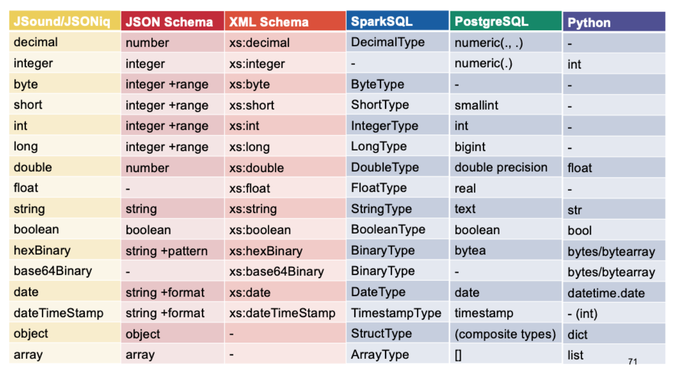
Item types

Also, all atomic types have in common that they have a logical value space and a lexical value space. Atomic types can be in a subtype relationship: a type is a subtype of another type if its logical value space is a subset of the latter.
However, in modern databases, it is customary to support unbounded integers.
Decimals correspond to real numbers that can be written as a finite sequence of digits in base 10, with an optional decimal period.Support for the entire decimal value space can be costly in performance. In order to address this issue, a floating-point standard (IEEE 754) was invented and is still very popular today.
Timestamp values are typically stored as longs (64-bit integers) expressing the number of milliseconds elapsed since January 1, 1970 by convention.
XML Schema, JSound and JSONiq follow the ISO 8601 standard.
The lexical representation of duration can vary, but there is a standard defined by ISO 8601 as well, starting with a P and prefixing sub-day parts with a T.
Maps (not be confused with records, which are similar) are maps from any atomic value to any value, i.e., generalize objects to keys that are not necessarily strings (e.g., numbers, dates, etc). However, unlike records, the type of the values must be the same for all keys.

JSound and JSON Schema

JSound is a schema language that was designed to be simple for 80% of the cases, making it particularly suitable in a teaching environment. It is independent of any programming language.
JSON Schema is another technology for validating JSON documents.
The type system of JSON Schema is thus less rich than that of JSound, but extra checks can be done with so-called formats, which include date, time, duration, email, and so on including generic regular expressions.
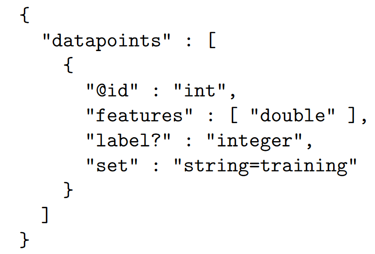
It is possible to require the presence of a key by adding an exclamation mark in JSound. in JSON Schema, which uses a “required” property associated with the list of required keys to express the same.
In the JSound compact syntax, extra keys are forbidden. Unlike JSound, in JSON Schema, extra properties are allowed by default. JSON Schema then allows to forbid extra properties with the “additionalProperties” property.
There are a few more features available in the compact JSound syntax (not in JSON Schema) with the special characters @, ? and =. The question mark (?) allows for null values (which are not the same as absent values). The arobase (@) indicates that one or more fields are primary keys for a list of objects that are members of the same array. The equal sign (=) is used to indicate a default value that is automatically populated if the value is absent.

Note that some values are quoted, which does not matter for validation: validation only checks whether lexical values are part of the type’s lexical space.

Accepting any values in JSound can be done with the type “item”, which contains all possible values. In JSON Schema, in order to declare a field to accept any values, you can use either true or an empty object in lieu of the type.

JSON Schema additionally allows to use false to forbid a field.

In JSON Schema, it is also possible to combine validation checks with Boolean combinations using “anyOf”.JSound schema allows defining unions of types with the vertical bar inside type strings.

In JSON Schema only (not in JSound), it is also possible to do a conjunction (logical and) with “allOf” as well as exclusive with “oneOf” as well as negation with “not”.

XML Schema

all elements in an XML Schema are in a namespace, the XML Schema namespace. The namespace is prescribed by the XML Schema standard and must be this one.

dataframe

There is a particular subclass of semi-structured datasets that are very interesting: valid datasets, which are collections of JSON objects valid against a common schema, with some requirements on the considered schemas. The datasets belonging to this particular subclass are called data frames, or dataframes.
relational tables are data frames, while data frames are not necessarily relational tables: data frames can be (and are often) nested, but they are still relatively homogeneous to some extent.Thus, Data frames are a generalization of (normalized) relational tables allowing for (organized and structured) nestedness.

data format

In fact, if the data is structured as a (valid) data frame, then there are many, many different formats that it can be stored in, and in a way that is much more efficient than JSON. These formats are highly optimized and typically stored in binary form, for example Parquet, Avro, Root, Google’s protocol buffers, etc.

Why is it possible to store the data more efficiently when it is valid and data-frame-friendly? One important reason is that the schema can be stored as a header in the binary format, and the data can be stored without repeating the fields in every record (as is done in textual JSON).

exercise

Dremel

Dremel is a query system developed at Google for deriving data stored in a nested data format such as XML, JSON, or Google Protocol Buffers into column storage, where it can be analyzed faster.

paper notes

Dynamo

CAP: AP.

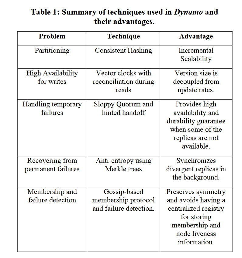
preference list and coordinator

A node handling a read or write operation is known as the coordinator. Typically, this is the first among the top N nodes in the preference list.

quorum-like system

To maintain consistency among its replicas, Dynamo uses a consistency protocol similar to those used in quorum systems. This protocol has two key configurable values: R and W. R is the minimum number of nodes that must participate in a successful read operation. W is the minimum number of nodes that must participate in a successful write operation. Setting R and W such that R + W > N yields a quorum-like system.

To remedy this it does not enforce strict quorum membership and instead it uses a “sloppy quorum”; all read and write operations are performed on the first N healthy nodes from the preference list.

Merkle Trees

A hash tree or Merkle tree is a binary tree in which every leaf node gets as its label a data block and every non-leaf node is labelled with the cryptographic hash of the labels of its child nodes. Some KeyValue stores use Merkle trees for efficiently detecting inconsistencies in data between replicas.

vector clock

Dremel

In contrast to layers such as Pig19 and Hive,16 it executes queries natively without translating them into MR jobs. Lastly, and importantly, Dremel uses a column-striped storage representation, which enables it to read less data from secondary storage and reduce CPU cost due to cheaper compression.

Repetition and definition levels

we define the repetition level as the number of repeated fields in the common prefix (including the first path element identifying the record). The definition level specifies the number of optional and repeated fields in the path (excluding the first path element).A definition level smaller than the maximal number of repeated and optional fields in a path denotes a NULL.

HDFS

Each block replica on a DataNode is represented by two files in the local host’s native file system. The first file contains the data itself and the second file is block’s metadata including checksums for the block data and the block’s generation stamp.

If the NameNode does not receive a heartbeat from a DataNode in ten minutes the NameNode considers the DataNode to be out of service and the block replicas hosted by that DataNode to be unavailable. The NameNode then schedules creation of new replicas of those blocks on other DataNodes. Heartbeats from a DataNode also carry information about total storage capacity, fraction of storage in use, and the number of data transfers currently in progress. These statistics are used for the NameNode’s space allocation and load balancing decisions. The NameNode does not directly call DataNodes. It uses replies to heartbeats to send instructions to the DataNodes.

A recently introduced feature of HDFS is the BackupNode. Like a CheckpointNode, the BackupNode is capable of creating periodic checkpoints, but in addition it maintains an inmemory, up-to-date image of the file system namespace that is always synchronized with the state of the NameNode.

A replica stored on a DataNode may become corrupted because of faults in memory, disk, or network. HDFS generates and stores checksums for each data block of an HDFS file. Checksums are verified by the HDFS client while reading to help detect any corruption caused either by client, DataNodes, or network. When a client creates an HDFS file, it computes the checksum sequence for each block and sends it to a DataNode along with the data. A DataNode stores checksums in a metadata file separate from the block’s data file. When HDFS reads a file, each block’s data and checksums are shipped to the client. The client computes the checksum for the received data and verifies that the newly computed checksums matches the checksums it received. If not, the client notifies the NameNode of the corrupt replica and then fetches a different replica of the block from another DataNode.

The design of HDFS I/O is particularly optimized for batch processing systems, like MapReduce, which require high throughput for sequential reads and writes.

Currently HDFS provides a configurable block placement policy interface so that the users and researchers can experiment and test any policy that’s optimal for their applications.

When a block becomes over replicated, the NameNode chooses a replica to remove. The NameNode will prefer not to reduce the number of racks that host replicas, and secondly prefer to remove a replica from the DataNode with the least amount of available disk space. When a block becomes under-replicated, it is put in the replication priority queue. A background thread periodically scans the head of the replication queue to decide where to place new replicas.

HDFS block placement strategy does not take into account DataNode disk space utilization. This is to avoid placing new—more likely to be referenced—data at a small subset of the DataNodes.

Each DataNode runs a block scanner that periodically scans its block replicas and verifies that stored checksums match the block data. Whenever a read client or a block scanner detects a corrupt block, it notifies the NameNode. The NameNode marks the replica as corrupt, but does not schedule deletion of the replica immediately. Instead, it starts to replicate a good copy of the block. Only when the good replica count reaches the replication factor of the block the corrupt replica is scheduled to be removed. So even if all replicas of a block are corrupt, the policy allows the user to retrieve its data from the corrupt replicas.

A present member of the cluster that becomes excluded is marked for decommissioning. Once a DataNode is marked as decommissioning, it will not be selected as the target of replica placement, but it will continue to serve read requests. The NameNode starts to schedule replication of its blocks to other DataNodes. Once the NameNode detects that all blocks on the decommissioning DataNode are replicated, the node enters the decommissioned state. Then it can be safely removed from the cluster without jeopardizing any data availability.

MapReduce

The master pings every worker periodically.If no response isrecei ved from awork er in acertain amount of time, the master marks the worker as failed.

json

JSON stands for JavaScript Object Notation and was inspired by the object literals of JavaScript.

A JSON value can be an object, array, number, string, true, false, or null.

The JSON syntax does not impose any restrictions on the strings used as names, does not require that name strings be unique, and does not assign any significance to the ordering of name/value pairs.

Numeric values that cannot be represented as sequences of digits (such as Infinity and NaN) are not permitted.

All strings in JSON must be double-quoted.

rumble

a query execution engine for large, heterogeneous, and nested collections of JSON objects built on top of Apache Spark.

xml

XML, unlike HTML, is case-sensitive. is not the same as or .

Every well-formed XML document has exactly one root element.

XML elements can have attributes. An attribute is a name-value pair attached to the element’s start-tag. Names are separated from values by an equals sign and optional whitespace. Values are enclosed in single or double quotation marks.

each element may have no more than one attribute with a given name.

Element and other XML names may contain essentially any alphanumeric character. This includes the standard English letters A through Z and a through z as well as the digits 0 through 9. They may also include these three punctuation characters: _ The underscore ,- The hyphen, . The period.Finally, all names beginning with the string “XML” (in any combination of case) are reserved for standardization in W3C XML-related specifications. XML names may only start with letters, ideograms, or the underscore character. They may not start with a number, hyphen, or period.

exam notes

2022

HTTP command and status code.
Storage type choosing.

HDFS and random access:
For distributed data storage though, and for the use case at hand where we read a large dataset, analyze it, and write back the output as a new dataset, random access is not needed. A distributed file system is designed so that, in cruise mode, its bottleneck will be the data flow (throughput), not the latency. This aspect of the design is directly consistent with a full-scan pattern, rather than with a random access pattern, the latter being strongly latency-bound.

json and comments:In JSON (JavaScript Object Notation), comments are not officially supported.

Hbase and meta table.
if empty json valid against to some schema.
mapreduce split.
mapreduce function: emit.
if reduce function can be used as combine function.

1NF,2NF and 3NF:
A candidate key is a minimal set of attributes that determines the other attributes included in the relation. A non-prime attribute is an attribute that is not part of the candidate key.Informally, the second normal form states that all attributes must depend on the entire candidate key.In other words, non-prime attributes must be functionally dependent on the key(s), but they must not depend on another non-prime attribute. 3NF non-prime attributes depend on “nothing but the key”.

different type comparision in mongodb.

If you have n dimensions, the CUBE operation will generate 2^n combinations.

xml schema:
You have already seen the xs:sequence element, which dictates that the elements it contains must appear in exactly the same order in which they appear within the sequence element.

mongdb atomic operations:
In MongoDB, a write operation is atomic on the level of a single document, even if the operation modifies multiple embedded documents within a single document.
When a single write operation (e.g. db.collection.updateMany()) modifies multiple documents, the modification of each document is atomic, but the operation as a whole is not atomic.

Json schema:
tuple validation.

references

https://vertabelo.com/blog/normalization-1nf-2nf-3nf/

On-Line Analytic Processing(OLAP)

On-Line Analytic Processing generally involves highly complex queries that use one or more aggregations.

OLAP and Data Warehouses

Data from many separate databases may be integrated into the warehouse. The warehouse is usually only updated overnight. Data warehouses play an important role in OLAP applications. First, the warehouse is necessary to organize and centralize data in a way that supports OLAP queries. Second, OLAP queries are usually complex and touching much of the data and take too much time to be executed in a transaction-processing system with high throughput requirements.

A Multidimensional View of OLAP Data

In typical OLAP applications there is a central relation or collection of data called the fact table. Often, it helps to think of the objects in the fact table as arranged in a multidimensional space. Two broad directions that have been taken by specialized systems that support cube-structured data for OLAP: ROLAP and MOLAP. ROLAP, which is Relational OLAP. In this approach, data may be stored in relations with a specialized structure called a “star schema”. MOLAP, which is Multidimensional OLAP. A specialized structure “data cude” is used to hold the data, including its aggregates.

Star Schemas

A star schema consists of the schema for the fact table, which links to several other relations, called “dimension tables”.

Slicing and Dicing

A choice of partition for each dimension “dices” the cude. The result is that the cude is divided into smaller cubes that represent groups of points whose statistics are aggregated by a query that performs this partitioning in its “group by” clause. Through the “where” clause, a query has the option of focusing on particular partitions alone one or more dimensions.(on a particular “slice” of the cube).

Data Cubes

The formal data cube precomputes all possible aggregates in a systematic way.

The Cube Operator

Given a fact table F, we can define an augmented table CUBE(F) that adds an additional value, denoted , to each dimension. The has the intuitive meaning “any,” and it represents aggregation along the dimension in which it appears.

The Cube Operator in SQL

SQL gives us a way to apply the cube operator within queries. If we add the term “WITH CUBE” to a group-by clause, then we get not only the tuple for each group, but also the tuples that represent aggregation along one or more of the dimensions along which we have grouped. These tuples appear in the result with NULL where we have used *.

However, SalesRollup would not contain tuples such as

Why graphs

Now, we do know a way to avoid joins and studied it at length: denormalizing the data to (homogeneous) collections of trees is a way of “pre-computing” the joins statically, so that the data is already joined (via nesting) at runtime.

Now, why is it efficient? Because doing down a tree only necessitates following pointers in memory. But trees cannot have cycles. Graph databases provide a way of generalizing the use in-memory pointers to traverse data to the general case in which cycles are present: this is called “index-free adjacency.”

Kinds of graph databases

There are many different graph database system products on the market, and they can be classified along several dimensions: Labeled property graph model vs. triple stores;Read-intensive vs. write-intensive;Local vs. distributed;Native vs. non-native.

Graph data models

Labeled property graphs

Computer scientists need to go one step further and also design how to store graphs physically. One way of doing so is to create an associative array mapping each node to the list of nodes that it connects to via an edge (adjacency lists). Another storage form is with an adjacency matrix: each row and each column represent a node, and a 0 or a 1 indicate the absence or presence of an edge between the row node and the column node.

Now, this does not quite work for us, because labeled property graphs enhance mathematical graphs with extra ingredients: properties, and labels.
how to “convert” a relational table to a labeled property graph: labels can be seen as table names, nodes as records, and properties as the attribute values for the records. This shows that relational tables can be physically stored as labeled property graphs. Of course, this does not work the other way round: given a graph, it will often not be possible to convert it “back” to a table in this specific way.

Triple stores

Triple stores are a different and simpler model. It views the graph as nodes and edges that all have labels, but without any properties. The graph is then represented as a list of edges, where each edge is a triple with the label of the origin node (called the subject), the label of the edge (called the property), and the label of the destination node (called the object).

Triple stores typically provide SPARQL capabilities to reason about and stored RDF data.

Querying graph data

We will now have a look at query languages for querying graphs, with a focus on Cypher, which is neo4j’s query language.

Cypher Philosophy

Cypher enables a user (or an application acting on behalf of a user) to ask the database to find data that matches a specific pattern. Colloquially, we ask the database to “find things like this.” And the way we describe what “things like this” look like is to draw them, using ASCII art.

Like most query languages, Cypher is composed of clauses. The simplest queries consist of a MATCH clause followed by a RETURN clause. There are other clauses we can use in a Cypher query: WHERE,WITH…AS…,CREATE,MERGE,DELETE,SET,UNION,FORWACH and so on.

A Comparison of Relational and Graph Modeling

Relational databases—with their rigid schemas and complex modeling characteristics—are not an especially good tool for supporting rapid change. What we need is a model that is closely aligned with the domain, but that doesn’t sacrifice performance, and that supports evolution while maintaining the integrity of the data as it undergoes rapid change and growth. That model is the graph model.

creating a graph

In practice, we tend to use CREATE when we’re adding to the graph and don’t mind duplication, and MERGE when duplication is not permitted by the domain.

Beginning a Query

In Cypher we always begin our queries from one or more well-known starting points in the graph—what are called bound nodes. Cypher uses any labels and property predicates supplied in the MATCH and WHERE clauses, together with metadata supplied by indexes and constraints, to find the starting points that anchor our graph patterns.

INDEXES AND CONSTRAINTS

To support efficient node lookup, Cypher allows us to create indexes per label and property combinations. For unique property values we can also specify constraints that assure uniqueness.

Neo4j

Neo4j is a graph database with native processing capabilities as well as native graph storage.

Native Graph Processing

Of the many different engine architectures, we say that a graph database has native processing capabilities if it exhibits a property called index-free adjacency.

A database engine that utilizes index-free adjacency is one in which each node maintains direct references to its adjacent nodes. Each node, therefore, acts as a micro-index of other nearby nodes, which is much cheaper than using global indexes. It means that query times are independent of the total size of the graph, and are instead simply proportional to the amount of the graph searched. A nonnative graph database engine, in contrast, uses (global) indexes to link nodes together.

Proponents for native graph processing argue that index-free adjacency is crucial for fast, efficient graph traversals. To understand why native graph processing is so much more efficient than graphs based on heavy indexing, consider the following. Depending on the implementation, index lookups could be O(log n) in algorithmic complexity versus O(1) for looking up immediate relationships. To traverse a network of m steps, the cost of the indexed approach, at O(m log n), dwarfs the cost of O(m) for an implementation that uses index-free adjacency.

Native Graph Storage

Neo4j stores graph data in a number of different store files. Each store file contains the data for a specific part of the graph (e.g., there are separate stores for nodes, relationships, labels, and properties).The division of storage responsibilities—particularly the separation of graph structure from property data—facilitates performant graph traversals, even though it means the user’s view of their graph and the actual records on disk are structurally dissimilar.

Like most of the Neo4j store files, the node store is a fixed-size record store, where each record is nine bytes in length. Fixed-size records enable fast lookups for nodes in the store file. If we have a node with id 100, then we know its record begins 900 bytes into the file. Based on this format, the database can directly compute a record’s location, at cost O(1), rather than performing a search, which would be cost O(log n).

Transactions

Transactions in Neo4j are semantically identical to traditional database transactions. Writes occur within a transaction context, with write locks being taken for consistency purposes on any nodes and relationships involved in the transaction. On successful completion of the transaction, changes are flushed to disk for durability, and the write locks released. These actions maintain the atomicity guarantees of the transaction.

CORE API, TRAVERSAL FRAMEWORK, OR CYPHER?

The Core API allows developers to fine-tune their queries so that they exhibit high affinity with the underlying graph. A well-written Core API query is often faster than any other approach. The downside is that such queries can be verbose, requiring considerable developer effort. Moreover, their high affinity with the underlying graph makes them tightly coupled to its structure. When the graph structure changes, they can often break. Cypher can be more tolerant of structural changes—things such as variable-length paths help mitigate variation and change.

The Traversal Framework is both more loosely coupled than the Core API (because it allows the developer to declare informational goals), and less verbose, and as a result a query written using the Traversal Framework typically requires less developer effort than the equivalent written using the Core API. Because it is a general-purpose framework, however, the Traversal Framework tends to perform marginally less well than a well-written Core API query.

exercise

Neo4j system design is different from mongodb on the consistency. MongoDB is eventually consistent, but neo4j is strong consistency and obey the ACID rules.

Cypher: note that label and property are case sensitive but the clause is not case sensitive.

RDF: Turtle Syntax

Mannual grouping and grouping sets: need to know how to translate between them.
grouping with rollup: rollup(c1,c2,c3) is equal to grouping sets((c1,c2,c3),(c1,c2),(c1),()). The ordering is important.

difference between neo4j and RDF:
Data Model:
Neo4j: Neo4j is a graph database that uses the property graph data model. In this model, nodes represent entities, relationships represent connections between entities, and both nodes and relationships can have key-value pairs as properties.
RDF: RDF is a data model for representing knowledge in the form of subject-predicate-object triples. Each triple represents a statement, and these triples can be used to build a graph of linked data. RDF is more abstract and can be implemented using various storage formats.

Query Language:
Neo4j: Neo4j uses the Cypher query language, which is specifically designed for querying graph databases. Cypher allows users to express graph patterns and relationships in a concise and readable manner.
RDF: RDF data is typically queried using SPARQL (SPARQL Protocol and RDF Query Language). SPARQL is a query language for querying and manipulating RDF data, and it provides powerful capabilities for navigating the graph structure.

Graph Structure:
Neo4j: In Neo4j, the graph is explicit, with nodes, relationships, and properties forming a connected graph structure. The focus is on relationships between entities and their properties.
RDF: RDF represents a graph, but the graph structure is more implicit. Resources are identified by URIs, and relationships are expressed through triples, allowing for the creation of a distributed and linked data web.

Schema:
Neo4j: Neo4j supports a flexible schema where nodes and relationships can have dynamic properties. While it provides some level of schema flexibility, users can define constraints and indexes to enforce certain structures.
RDF: RDF is schema-agnostic, allowing for more dynamic and extensible data representation. Schemas can be defined using RDF vocabularies and ontologies, such as RDFS and OWL.

Use Cases:
Neo4j: Neo4j is often used for applications where relationships and graph structures are central, such as social networks, recommendation engines, and network analysis.
RDF: RDF is commonly used in the context of the Semantic Web for representing and linking diverse data sources, allowing for interoperability and knowledge representation.

references

Robinson, I. et al. (2015). Graph Databases (2nd ed.)

model-based reinforcement learning

We face three main challenges in model-based reinforcement learning. First, given a fixed model, we need to perform planning to decide on which actions to play. Second, we need to learn models f and r accurately and efficiently. Third, we need to effectively trade exploration and exploitation.

Planning

Deterministic Dynamics

To begin with, let us assume that our dynamics model is deterministic and known. That is, given a state-action pair, we know the subsequent state.

Model-free Approximate Reinforcement Learning

Tabular Reinforcement Learning as Optimization

In particular, in the tabular setting (i.e., over a discrete domain), we can parameterize the value function exactly by learning a separate parameter for each state.

Now, we cannot compute this derivative because we cannot compute the expectation. Firstly, the expectation is over the true value function which is unknown to us. Secondly, the expectation is over the transition model which we are trying to avoid in model-free methods. To resolve the first issue, analogously to TD-learning, instead of learning the true value function vπ which is unknown, we learn the bootstrapping estimate Vπ. To resolve the first issue, analogously to TD-learning, instead of learning the true value function vπ which is unknown, we learn the bootstrapping estimate Vπ. we will use a Monte Carlo estimate using a single sample. Recall that this is only possible because the transitions are conditionally independent given the state-action pair.

Therefore, TD-learning is essentially performing stochastic gradient descent using the TD-error as an unbiased gradient estimate.
Stochastic gradient descent with a bootstrapping estimate is also called stochastic semi-gradient descent.

Value Function Approximation

Our goal for large state-action spaces is to exploit the smoothness properties5 of the value function to condense the representation.

Heuristics

The vanilla stochastic semi-gradient descent is very slow.
There are mainly two problems.
As we are trying to learn an approximate value function that depends on the bootstrapping estimate, this means that the optimization target is “moving” between iterations. In practice, moving targets lead to stability issues. One such technique aiming to “stabilize” the optimization targets is called neural fitted Q-iteration or deep Q-networks (DQN). DQN updates the neural network used for the approximate bootstrapping estimate infrequently to maintain a constant optimization target across multiple episodes. One approach is to clone the neural network and maintain one changing neural network (“online network”) for the most recent estimate of the Q-function which is parameterized by θ, and one fixed neural network (“target network”) used as the target which is parameterized by θold and which is updated infrequently.

This technique is known as experience replay. Another approach is Polyak averaging where the target network is gradually “nudged” by the neural network used to estimate the Q function.

Now, observe that the estimates Q⋆ are noisy estimates of q⋆. The fact that the update rules can be affected by inaccuracies (i.e., noise in the estimates) of the learned Q-function is known as the “maximization bias”. Double DQN (DDQN) is an algorithm that addresses this maximization bias. Instead of picking the optimal action with respect to the old network, it picks the optimal action with respect to the new network. Intuitively, this change ensures that the evaluation of the target network is consistent with the updated Q-function, which makes it more difficult for the algorithm to be affected by noise.

Policy Approximation

Methods that find an approximate policy are also called policy search methods or policy gradient methods. Policy gradient methods use randomized policies for encouraging exploration.

Estimating Policy Values

The policy value function measures the expected discounted payoff of policy π.

Reinforce Gradient

In this context, however, we cannot apply the reparameterization trick. Fortunately, there is another way of estimating this gradient.

When using a neural network for the parameterization of the policy π, we can use automatic differentiation to obtain unbiased gradient estimates. However, it turns out that the variance of these estimates is very large. Using so-called baselines can reduce the variance dramatically.

The baseline essentially captures the expected or average value, providing a reference point. By subtracting this reference point, the updates become more focused on the deviations from the expected values, which can reduce the variance in these deviations.

Typically, policy gradient methods are slow due to the large variance in the score gradient estimates. Because of this, they need to take small steps and require many rollouts of a Markov chain. Moreover, we cannot reuse data from previous rollouts, as policy gradient methods are fundamentally on-policy.

Actor-Critic Methods

Actor-Critic methods reduce the variance of policy gradient estimates by using ideas from value function approximation. They use function approximation both to approximate value functions and to approximate policies.

Advantage Function

Intuitively, the advantage function is a shifted version of the state-action function q that is relative to 0. It turns out that using this quantity instead, has numerical advantages.

Policy Gradient Theorem

Intuitively, ρθ(x) measures how often we visit state x when following policy πθ. It can be thought of as a “discounted frequency”. Importantly, ρθ is not a probability distribution, as it is not normalized to integrate to 1. Instead, ρθ is what is often called a finite measure. Therefore, eq. (12.57) is not a real expectation!

On-policy Actor-Critics

OAC

Due to the use of TD-learning for learning the critic, this algorithm is fundamentally on-policy.

A2C

that the Q-function is an absolute quantity, whereas the advantage function is a relative quantity, where the sign is informative for the gradient direction. Intuitively, an absolute value is harder to estimate than the sign. Actor-Critic methods are therefore often implemented with respect to the advantage function rather than the Q-function.

GAE/GAAE

Taking a step back, observe that the policy gradient methods such as REINFORCE generally have high variance in their gradient estimates. However, due to using Monte Carlo estimates of Gt, the gradient estimates are unbiased. In contrast, using a bootstrapped Q-function to obtain gradient estimates yields estimates with a smaller variance, but those estimates are biased. We are therefore faced with a bias-variance tradeoff. A natural approach is therefore to blend both gradient estimates to allow for effectively trading bias and variance. This leads to algorithms such as generalized advantage estimation (GAE/GAAE).

Improving sample efficiency(TRPO/PPO)

Actor-Critic methods generally suffer from low sample efficiency. One well-known variant that slightly improves the sample efficiency is trust-region policy optimization (TRPO).

Intuitively, taking the expectation with respect to the previous policy πθk , means that we can reuse data from rollouts within the same iteration. TRPO allows reusing past data as long as it can still be “trusted”. This makes TRPO “somewhat” off-policy. Fundamentally, though, TRPO is still an on-policy method. Proximal policy optimization (PPO) is a heuristic variant of TRPO that often works well in practice.

Off-policy Actor-Critics

These algorithms use the reparameterization gradient estimates, instead of score gradient estimators.

DDPG

As our method is off-policy, a simple idea in continuous action spaces is to add Gaussian noise to the action selected by πθ — also known as Gaussian noise “dithering”. This corresponds to an algorithm called deep deterministic policy gradients.
This algorithm is essentially equivalent to Q-learning with function approximation (e.g., DQN), with the only exception that we replace the maximization over actions with the learned policy πθ.

Twin delayed DDPG (TD3) is an extension of DDPG that uses two separate critic networks for predicting the maximum action and evaluating the policy. This addresses the maximization bias akin to Double-DQN. TD3 also applies delayed updates to the actor network, which increases stability.

Off-Policy Actor Critics with Randomized Policies

The algorithm that uses eq. (12.81) to obtain gradients for the critic and reparameterization gradients for the actor is called stochastic value gradients (SVG).

Off-policy Actor-Critics with Entropy Regularization

In practice, algorithms like SVG often do not explore enough. A key issue with relying on randomized policies for exploration is that they might collapse to deterministic policies.

A simple trick that encourages a little bit of extra exploration is to regularize the randomized policies “away” from putting all mass on a single action. This approach is known as entropy regularization and it leads to an analogue of Markov decision processes called entropy-regularized Markov decision process, where suitably defined regularized state-action value functions (so-called soft value functions) are used.

soft actor critic(SAC)

references

https://towardsdatascience.com/soft-actor-critic-demystified-b8427df61665
https://github.com/tsmatz/reinforcement-learning-tutorials/blob/master/06-sac.ipynb
https://spinningup.openai.com/en/latest/algorithms/sac.html
https://towardsdatascience.com/policy-gradients-in-a-nutshell-8b72f9743c5d
https://lilianweng.github.io/posts/2018-04-08-policy-gradient/

Querying denormalized data

imperative vs declarative

Imperative programming is a programming paradigm that expresses computation as a series of statements that change a program’s state. In imperative programming, the focus is on describing how a program operates step by step. Common imperative languages include C, C++, Java, and Python.

In contrast to imperative programming, declarative programming focuses on describing what the program should accomplish rather than how to achieve it. In a declarative host language, the emphasis is on specifying the desired outcome or properties, and the language itself takes care of the underlying implementation details. Such as SQL, HTML.

motivation

Denormalized data

it is characterized with two features: nestedness, and heterogeneity. In fact, denormalized datasets should not be seen as “broken tables pushed to their limits”, but rather as collections of trees.

Features of a query language

A query language for datasets has three main features: Declarative, Functional, and Set-based. First, it is declarative. This means that the users do not focus on how the query is computed, but on what it should return. Being functional means that the query language is made of composable expressions that nest with each other, like a Lego game. Finally, it is set-based, in the sense that the values taken and returned by expressions are not only single values (scalars), but are large sequences of items (in the case of SQL, an item is a row).

Query languages for denormalized data

For denormalized data though, sadly, the number of languages keeps increasing: the oldest ones being XQuery, JSONiq, but then now also JMESPath, SpahQL, JSON Query, PartiQL, UnQL, N1QL, ObjectPath, JSONPath, ArangoDB Query Language (AQL), SQL++, GraphQL, MRQL, Asterix Query Language (AQL), RQL.

JSONiq as a data calculator

it can perform arithmetics, but also comparison and logic. It is, however, more powerful than a common calculator and supports more complex constructs, for example variable binding.
It also supports all JSON values. Any copy-pasted JSON value literally returns itself.
And, unlike a calculator, it can access storage.

The JSONiq Data Model

Every expression of the JSONiq “data calculator” returns a sequence of items.An item can be either an object, an array, an atomic item, or a function item. A sequence can also be empty. Caution, the empty sequence is not the same logically as a null item.

Navigation

The general idea of navigation is that it is possible to “dive” into the nested data with dots and square brackets (originally, these were slashes with XPath) – all in parallel: starting with an original collection of objects (or, possibly, a single document), each step (i.e., for each dot and each pair of square brackets) goes down the nested structure and returns another sequence of nested items.

Object lookups (dot syntax)

json-doc(“file.json”).o

Array unboxing (empty square bracket syntax)

We can unbox the array, meaning, extract its members as a sequence of seven object items, with empty square brackets.json-doc(“file.json”).o[].

Parallel navigation

The dot syntax, in fact, works on sequences, too and will extract the value associated with a key in every object of the sequence (anything else than an object is ignored and thrown away).

Filtering with predicates (simple square bracket syntax)

It is possible to filter any sequence with a predicate, where $in the predicate refers to the current item being tested. json-doc("file.json").o[].a.b[][$.c = 3].It is also possible to access the item at position n in a sequence with this same notation: json-doc(“file.json”).o[].a.b[][5].

Array lookup (double square bracket syntax)

To access the n-th member of an array, you can use double-squarebrackets, like so:
json-doc(“file.json”).o[[2]].a.

A common pitfall: Array lookup vs. Sequence predicates

Do not confuse sequence positions (single square brackets) with array positions (double square brackets)!
([1, 2], [3, 4])[2] -> [ 3, 4 ]
([1, 2], [3, 4])[[2]] -> 2 4

Schema discovery

Collections

many datasets are in fact found in the form of large collections of smaller objects (as in document stores). Such collections are access with a function call together with a name or (if reading from a data lake) a path.

Getting all top-level keys

The keys function retrieves all keys. It can be called on the entire sequence of objects and will return all unique keys found (at the top level) in that collection.

Getting unique values associated with a key

With distinct-values, it is then possible to eliminate duplicates and look at unique values:
distinct-values(collection( “https://www.rumbledb.org/samples/git-archive.jsonl“ ).type)

Aggregations

Aggregations can be made on entire sequences with a single function call:The five basic functions are count, sum, avg, min, max.
count(distinct-values(collection( “https://www.rumbledb.org/samples/git-archive.jsonl“ ).type))

Construction

Construction of atomic values

Atomic values that are core to JSON can be constructed with exactly the same syntax as JSON.

Construction of objects and arrays

In fact, one can copy-paste any JSON value, and it will always be recognized as a valid JSONiq query returning that value.

Construction of sequences

Sequences can be constructed (and concatenated) using commas.Increasing sequences of integers can also be built with the to keyword.

Scalar expressions

Sequences of items can have any number of items. A few JSONiq expression (arithmetic, logic, value comparison…) work on the particular case that a sequence has zero or one items.

Arithmetic

JSONiq supports basic arithmetic: addition (+), subtraction (-), division (div), integer division (idiv) and modulo (mod).If the data types are different, then conversions are made automatically. The empty sequence enjoys special treatment: if one of the sides (or both) is the empty sequence, then the arithmetic expression returns an empty sequence (no error). If one of the two sides is null (and the other side is not the empty sequence), then the arithmetic expression returns null. If one of the sides (or both) is not a number, null, or the empty sequence, then a type error is thrown.

String manipulation

String concatenation is done with a double vertical bar: “foo” || “bar”.
Most other string manipulation primitives are available from the rich JSONiq builtin function library:
concat(“foo”, “bar”),string-join((“foo”, “bar”, “foobar”), “-“),substr(“foobar”, 4, 3),
string-length(“foobar”).

Value comparison

Sequences of one atomic item can be compared with eq (equal), ne (not equal), le (lower or equal), gt (greater or equal), lt (lower than) and gt (greater than).

Logic

JSONiq supports the three basic logic expressions and, or, and not. not has the highest precedence, then and, then or.
JSONiq also supports universal and existential quantification:
every $i in 1 to 10 satisfies $i gt 0, some $i in 1 to 10 satisfies $i gt 5.

If one of the two sides is not a sequence of a single Boolean item, then implicit conversions are made. This mechanism is called the Effective Boolean Value (EBV). For example, an empty sequence, or a sequence of one empty string, or a sequence of one zero integer, is considered false. A sequence of one non-empty string, or a sequence or one non-zero integer, or a sequence starting with one object (or array) is considered true.

General comparison

JSONiq has a shortcut for existential quantification on value comparisons. This is called general comparison.

some $i in (1, 2, 3, 4, 5) satisfies $i eq 1 ==
(1, 2, 3, 4, 5) = 1.

Composability

Data flow

A few expressions give some control over the data flow by picking the output or this or that expression based on the value of another expression. This includes conditional expressions. This includes conditional expressions. This also includes try-catch expressions.

Binding variables with cascades of let clauses

Variables in JSONiq start with a dollar sign. It is important to understand that this is not a variable assignment that would change the value of a variable. This is only a declarative binding.

FLWOR expressions

One of the most important and powerful features of JSONiq is the FLWOR expression. It corresponds to SELECT-FROM-WHERE queries in SQL, however, it is considerably more expressive and generic than them in several aspects. In JSONiq the clauses can appear in any order with the exception of the first and last clause. JSONiq supports a let clause, which does not exist in SQL.
In SQL, when iterating over multiple tables in the FROM clause, they “do not see each other”. In JSONiq, for clauses (which correspond to FROM clauses in SQL), do see each other, meaning that it is possible to iterate in higher and higher levels of nesting by referring to a previous for variable.

For clauses

It can thus be seen that the for clause is akin to the FROM clause in SQL, and the return is akin to the SELECT clause. Projection in JSONiq can be made with a project() function call, with the keys to keep. It is possible to implement a join with a sequence of two for clauses and a predicate. Note that allowing empty can be used to perform a left outer join, i.e., to account for the case when there are no matching records in the second collection.

Let clauses

A let clause outputs exactly one outgoing tuple for each incoming tuple (think of a map transformation in Spark). Let clauses also allow for joining the two datasets.

Where clauses

Where clauses are used to filter variable bindings (tuples) based on a predicate on these variables. They are the equivalent to a WHERE clause in SQL.

Order by clauses

Order by clauses are used to reorganize the order of the tuples, but without altering them. They are the same as ORDER BY clauses in SQL.It is also possible, like in SQL, to specify an ascending or a descending order. In case of ties between tuples, the order is arbitrary. But it is possible to sort on another variable in case there is a tie with the first one (compound sorting keys). It is possible to control what to do with empty sequences: they can be considered smallest or greatest.

Group by clauses

Group by clauses organize tuples in groups based on matching keys, and then output only one tuple for each group, aggregating other variables (count, sum, max, min…). It is also possible to opt out of aggregating other (non-grouping-key) variables.

Types

Variable types

Since every value in JSONiq is a sequence of item, a sequence type consists of two parts: an item type, and a cardinality.
Item types can be any of the builtin atomic types. as well as “object”, “array” and the most generic item type, “item”.
Cardinality can be one of the following four:Any number of items (suffix ); for example object, One or more items (suffix +); for example array+,Zero or one item (suffix ?); for example integer,Exactly one item (no suffix); for example boolean?

Type expressions

An “instance of” expression checks whether a sequences matches a sequence type, and returns true or false. A “cast as” expression casts single items to an expected item type.
A “castable as” expression tests whether a cast would succeed (in which case it returns true) or not (false).
A “treat as” expression checks whether its input sequence matches an expected type (like a type on a variable); if it does, the input sequence is returned unchanged. If not, an error is raised.

Types in user-defined functions

JSONiq supports user-defined functions. Parameter types can be optionally specified, and a return type can also be optionally specified.

Validating against a schema

It is possible to declare a schema, associating it with a user-defined type, and to validate a sequence of items against this user-defined type.

Architecture of a query engine

Static phase

When a query is received by an engine, it is text that needs to be parsed. The output of this is a tree structure called an Abstract Syntax Tree. An Abstract Syntax Tree, even though it already has the structure of a tree, is tightly tied to the original syntax. Thus, it needs to be converted into a more abstract Intermediate Representation called an expression tree. Every node in this tree corresponds to either an expression or a clause in the JSONiq language, making the design modular. At this point, static typing takes place, meaning that the engine infers the static type of each expression, that is, the most specific type possible expected at runtime (but without actually running the program). Engines like RumbleDB perform their optimization round on this Intermediate Representation. Once optimizations have been done, RumbleDB decides the mode with which each expression and clause will be evaluated (locally, sequentially, in parallel, in DataFrames, etc). The resulting expression tree is then converted to a runtime iterator tree; this is the query plan that will actually be evaluated by the engine.

Dynamic phase

During the dynamic phase, the root of the tree is asked to produce a sequence of items, which is to be the final output of the query as a whole. Then, recursively, each node in the tree will ask its children to produce sequences of items (or tuple streams). Each node then combines the sequences of items (or tuple streams) it receives from its children in order to produce its own sequence of items according to its semantics, and pass it to its parent.

Materialization

When a sequence of items is materialized, it means that an actual List (or Array, or Vector), native to the language of implementation (in this case Java) is stored in local memory, filled with the items.

Streaming

When a sequence of items (or tuple stream) is produced and consumed in a streaming fashion, it means that the items (or tuples) are produced and consumed one by one, iteratively. But the whole sequence of items (or tuple stream) is never stored anywhere. The classical pattern for doing so is known as the Volcano iterator architecture.

However, there are two problems with this: first, it can take a lot of time to go through the entire sequence (imagine doing so with billions or trillions of items). Second, there are expressions or clauses that are not compatible with streaming (consider, for example, the group by or order by clause, which cannot be implemented without materializing their full input).

Parallel execution (with RDDs)

When a sequence becomes unreasonably large, RumbleDB switches to a parallel execution, leveraging Spark capabilities: the sequences of items are passed and processed as RDDs of Item objects.

Parallel execution (with DataFrames)

The RDD implementation supports heterogeneous sequences by leveraging the polymorphism of Item objects. However, this is not efficient in the case that Items in the same sequence happen to have a regular structure. Thus, if the Items in a sequence are valid against a specific schema, or even against an array type or an atomic type, the underlying physical storage in memory relies on Spark DataFrames instead of RDDs.

To summarize, homogeneous sequences of the most common types are stored in DataFrames, and RDDs are used in all other cases.

Parallel execution (with Native SQL)

In some cases (more in every release), RumbleDB is able to evaluate the query using only Spark SQL, compiling JSONiq to SQL directly instead of packing Java runtime iterators in UDFs. This leads to faster execution, because UDFs are slower than a native execution in SQL. This is because, to a SQL optimizer, UDFs are opaque and prevent automatic optimizations.

Document stores

Can we rebuild a similar system for collections of trees, in the sense that we drop all three constraints: relational integrity, domain integrity, and atomic integrity? Document stores bring us one step in this direction.

Challenges

Schema on read

In a relational database management system, it is not possible to populate a table without having defined its schema first. However, when encountering such denormalized data, in the real world, there is often no schema. In fact, one of the important features of a system that deals with denormalized data is the ability to discover a schema.

Making trees fit in tables

Several XML elements (or, likewise, several JSON objects) can be naturally mapped to a relational table with several rows if the collection is flat and homogeneous, but semi-structured data can generally be nested and heterogeneous. if we map nested and heterogeneous into a table,such mapping will at best have to be done for every single dataset, and requires in most cases a schema, whereas we are looking for a generic solution for semistructured data with no a-priori schema information.

Document stores

Document stores provide a native database management system for semi-structured data. Document stores work on collections of records, generalizing the way that relational tables can be seen as collections of rows. It is important to understand that document stores are optimized for the typical use cases of many records of small to medium sizes. Typically, a collection can have millions or billions of documents, while each single document weighs no more than 16 MB (or a size in a similar magnitude). Finally, a collection of documents need not have a schema: it is possible to insert random documents that have dissimilar structures with no problem at all. Most document stores, however, do provide the ability to add a schema. Document stores can generally do selection, projection, aggregation and sorting quite well, but many of them are typically not (yet) optimized for joining collections. In fact, often, their language or API does not offer any joining functionality at all, which pushes the burden to reimplement joins in a host language to the users. This is a serious breach of data independence.

Implementations

There is a very large number of products in the document store space for both JSON and XML, let us mention for example MongoDB, CouchDB, ElasticSearch, Cloudant, existDB, ArangoDB, BaseX, MarkLogic, DocumentDB, CosmosDB, and so on. We will focus, as an example, on MongoDB.

Physical storage

Just like the storage format is optimized for tabular data in a relational database management system, it is optimized for tree-like data in a document store. In MongoDB, the format is a binary version of JSON called BSON. BSON is basically based on a sequence of tokens that efficiently encode the JSON constructs found in a document. The immediate benefit of BSON is that it takes less space in storage than JSON stored as a text file: for example, null, true and false literals need four or five bytes in text format at best, while they can be efficiently encoded as single bytes in BSON. Furthermore, BSON supports additional types that JSON does not have, such as dates.

Querying paradigm (CRUD)

The API of MongoDB, like many document stores, is based on the CRUD paradigm. CRUD means Create, Read, Update, Delete and corresponds to low-level primitives similar to those for HBase. MongoDB supports several host languages to query collections via an API. This includes in particular JavaScript and Python, but many other languages are supported via drivers. We will use JavaScript here because this is the native host language of MongoDB. It is important to note that these APIs are not query languages. MongoDB also provides access to the data via a shall called mongo or, newly, mongosh. This is a simple JavaScript interface wrapped around the MongoDB’s node.js driver.

Populating a collection

To create a collection, one can simply insert a document in it, and it will be automatically created if it does not exist.

MongoDB automatically adds to every inserted document a special field called “ id” and associated with a value called an Object ID and with a type of its own.Object IDs are convenient for deleting or updating a specific document with no ambiguity.

Querying a collection

Scan a collection

Asking for the contents of an entire collection is done with a simple find() call on the previous object:db.collection.find().This function does not in fact return the entire collection; rather, it returns some pointer, called a cursor, to the collection; the user can then iterate on the cursor in an imperative fashion in the host language.

Selection

It is possible to perform a selection on a collection by passing a parameter to find() that is a JSON object:
db.collection.find({ “Theory” : “Relativity” }).

A disjunction (OR) uses a special MongoDB keyword, prefixed with a dollar sign:
db.collection.find( { “$or” : [ { “Theory”:”Relativity” }, { “Last”:”Einstein” } ] } ).

MongoDB offers many other keywords, for example for comparison other than equality:
db.collection.find( { “Publications” : { “$gte” : 100 } } )

Projection

Projections are made with the second parameter of this same find() method. This is done in form of a JSON object associating all the desired keys in the projection with the value 1. db.scientists.find( { “Theory” : “Relativity” }, { “First” : 1, “Last”: 1 } ).

It is also possible to project fields away in the same way with 0s, however 1s and 0s cannot be mixed in the projection parameter, except in the specific above case of projecting away the object ID

Counting

Counting can be done by chaining a count() method call:
db.scientists.find( { “Theory” : “Relativity” } ).count().

Sorting

Sorting can be done by chaining a sort() method call.
db.scientists.find( { “Theory” : “Relativity” }, { “First” : 1, “Last” : 1 } ).sort( { “First” : 1, “Name” : -1 } )

1 is for ascending order and -1 for descending order.It is also possible to add limits and offsets to paginate results also by chaining more method calls:
db.scientists.find( { “Theory” : “Relativity” }, { “First” : 1, “Last” : 1 } ).sort( { “First” : 1, “Name” : -1 } ).skip(30).limit(10).

Note that, contrary to intuition, the order of the calls does not matter, as this is really just the creation of a query plan by providing parameters (in any order).

Duplicate elimination

It is possible to obtain all the distinct values for one field with a distinct() call: db.scientists.distinct(“Theory”)

Querying for heterogeneity

Absent fields

Absent fields can be filtered with: db.scientists.find( { “Theory” : null } ).

Filtering for values across types

db.collection.find( { “$or” : [ { “Theory”: “Relativity” }, { “Theory”: 42 }, { “Theory”: null } ] } )

db.scientists.find( { “Theory” : { “$in” : [“Relativity”, 42, null ] } } ).

MongoDB is also able to sort on fields that have heterogeneous data types. It does so by first order by type in some (arbitrary, but documented) order, and then within each type.

Querying for nestedness

Nestedness in MongoDB is handled in several ad-hoc ways for specific use cases.

Values in nested objects

We saw how to select documents based on values associated with a top-level keys. What about values that are not at the top-level, but in nested objects?
The first solution that might come to mind is something like this: db.scientists.find({ “Name” : { “First” : “Albert” } }) However, this query will not have the behavior many would have expected: instead of finding documents that have a value “Albert” associated with the key “First” in an object itself associated with the top-level key ”Name”, this query looks for an exact match of the entire object.
In order to include documents such as above, MongoDB uses a dot syntax: db.scientists.find({ “Name.First” : “Albert” }).

Values in nested arrays

MongoDB allows to filter documents based on whether a nested array contains a specific value, like so: db.scientists.find({ “Theories” : “Special relativity” }).

Deleting objects from a collection

Objects can be deleted from a collection either one at a time with deleteOne(), or several at a time with deleteMany(): db.scientists.deleteMany( { “century” : “15” } ).

Updating objects in a collection

Documents can be updated with updateOne() and updateMany() by providing both a filtering criterion (with the same syntax as the first parameter of find()) and an update to apply. The command looks like so: db.scientists.updateMany( { “Last” : “Einstein” }, { $set : { “Century” : “20” } } ).

The granularity of updates is per document, that is, a single document can be updated by at most one query at the same time.However, within the same collection, several different documents can be modified concurrently by different queries in parallel.

Complex pipelines

For grouping and such more complex queries, MongoDB provides an API in the form of aggregation pipelines.
db.scientists.aggregate( { $match : { “Century” : 20 }}, { $group : { “Year” : “$year”, “Count” : { “$sum” : 1 } } }, { $sort : { “Count” : -1 } }, { $limit : 5 } ).

Limitations of a document store querying API

Simple use cases are straightforward to handle, however more complex use cases require a lot of additional code in the host language, be it JavaScript or Python. An example is that joins must be taken care of by the end user in the host language: the burden of implementing more complex use cases is pushed to the end user.

Architecture

The architecture of MongoDB follows similar principles to what we covered before: scaling out the hardware to multiple machine, and sharding as well as replicating the data.

Sharding collections

Collections in MongoDB can be sharded. Shards are determined by selecting one or several fields. (Lexicographically-ordered) intervals over these fields then determine the shards. The fields used to shard must be organized in a tree index structure.

Replica sets

A replica set is a set of several nodes running the MongoDB server process. The nodes within the same replica set all have a copy of the same data.

Each shard of each collection is assigned to exactly one replica set. Note that this architecture is not the same as that of HDFS, in which the replicas are spread over the entire cluster with no notion of “walls” between replica sets and no two DataNodes having the exact same block replicas.

Write concerns

When writing (be it delete, update or insert) to a collection, more exactly, to a specific shard of a collection, MongoDB checks that a specific minimum number of nodes (within the replica set that is responsible for the shard) have successfully performed the update.

Motivation

A document store, unlike a data lake, manages the physical data layout. This has a cost: the need to import (ETL) data before it is possible to query it, but this cost comes with a nice benefit: index support, just like relational database management systems.

Hash indices

Hash indices are used to optimize point queries and more generally query that select on a specific value of a field. The general idea is that all the values that a field takes in a specific collection can be hashed to an integer. The value, together with pointers to the corresponding documents, is then placed in a physical array in memory, at the position corresponding to this integer.

Tree indices

Hash indices are great and fast, but have limitations: first, they consume space. The more one wants to avoid hash collisions, the larger the array needs to be. But more importantly, hash indices cannot support range queries. This is because hashes do not preserve the order of the values and distribute them “randomly” in the index array structure.

Range queries are supported with tree indices. Instead of an array, tree indices use some sort of tree structure in which they arrange the possible values of the indexed field, such that the values are ordered when traversing the tree in a depth-first-search manner. More precisely, the structure is called a B+-tree. Unlike a simple binary tree, nodes have a large number of children.

Secondary indices

By default, MongoDB always builds a tree index for the id field. Users can request to build hash and tree indices for more fields. These indices are called secondary indices.

The command for building a hash index looks like so: db.scientists.createIndex({ “Name.Last” : “hash” })

And for a tree index (1 means in ascending order, -1 would be descending): db.scientists.createIndex({ “Name.Last” : 1 }).

When are indices useful

When building indices, it is important to get a feeling for whether a query will be faster or not with this index.

index types

Single Field Indexes

By default, all collections have an index on the _id field. You can add additional indexes to speed up important queries and operations. You can create a single-field index on any field in a document, including:Top-level document fields, Embedded documents ,Fields within embedded documents. When you create an index on an embedded document, only queries that specify the entire embedded document use the index. Queries on a specific field within the document do not use the index. In order for a dot notation query to use an index, you must create an index on the specific embedded field you are querying, not the entire embedded object.

Compound Indexes

Compound indexes collect and sort data from two or more fields in each document in a collection. Data is grouped by the first field in the index and then by each subsequent field.

The order of the indexed fields impacts the effectiveness of a compound index. Compound indexes contain references to documents according to the order of the fields in the index. To create efficient compound indexes, follow the ESR (Equality, Sort, Range) rule. The ESR (Equality, Sort, Range) Rule is to place fields that require exact matches first in your index. Sort follows equality matches because the equality matches reduce the number of documents that need to be sorted. Sorting after the equality matches also allows MongoDB to do a non-blocking sort. “Range” filters scan fields. The scan doesn’t require an exact match, which means range filters are loosely bound to index keys. To improve query efficiency, make the range bounds as tight as possible and use equality matches to limit the number of documents that must be scanned. MongoDB cannot do an index sort on the results of a range filter. Place the range filter after the sort predicate so MongoDB can use a non-blocking index sort.

Compound indexes cannot support queries where the sort order does not match the index or the reverse of the index.

Index prefixes are the beginning subsets of indexed fields. Compound indexes support queries on all fields included in the index prefix. Index fields are parsed in order; if a query omits an index prefix, it is unable to use any index fields that follow that prefix.

Multikey Indexes

Multikey indexes collect and sort data from fields containing array values. Multikey indexes improve performance for queries on array fields.

In a compound multikey index, each indexed document can have at most one indexed field whose value is an array.

exercise

data model

Embedded Data Models

In general, embedding provides better performance for read operations, as well as the ability to request and retrieve related data in a single database operation. Embedded data models make it possible to update related data in a single atomic write operation.

Normalized Data Models

Normalized data models describe relationships using references between documents.

references

https://www.mongodb.com/docs/manual/core/data-model-design/

Tabular Reinforcement Learning

The Reinforcement Learning Problem

Reinforcement learning is concerned with probabilistic planning in unknown environments. In this chapter, we will begin by considering reinforcement learning with small state and action spaces. This setting is often called the tabular setting, as the value functions can be computed exhaustively for all states and stored in a table.

Clearly, the agent needs to trade exploring and learning about the environment with exploiting its knowledge to maximize rewards. In fact, Bayesian optimization can be viewed as reinforcement learning with a fixed state and a continuous action space: In each round, the agent plays an action, aiming to find the action that maximizes the reward.Another key challenge of reinforcement learning is that the observed data is dependent on the played actions.

Trajectories

Crucially, the newly observed states xt+1 and the rewards rt (across multiple transitions) are conditionally independent given the previous states xt and actions at. This independence property is crucial for being able to learn about the underlying Markov decision process. Notably, this implies that we can apply the law of large numbers (1.83) and Hoeffding’s inequality (1.87) to our estimators of both quantities.

The collection of data is commonly classified into two settings. In the episodic setting, the agent performs a sequence of “training” rounds (called episodes). In the beginning of each round, the agent is reset to some initial state. In contrast, in the continuous setting (or non-episodic,or online setting), the agent learns online.

control

Another important distinction in how data is collected, is the distinction between on-policy and off-policy control. As the names suggest, on-policy methods are used when the agent has control over its own actions, in other words, the agent can freely choose to follow any policy. In contrast, off-policy methods can be used even when the agent cannot freely choose its actions. Off-policy methods are therefore able to make use of observational data.Off-policy methods are therefore more sample-efficient than on-policy methods. This is crucial, especially in settings where conducting experiments (i.e., collecting new data) is expensive.

On-Policy learning algorithms are the algorithms that evaluate and improve the same policy which is being used to select actions. Off-Policy learning algorithms evaluate and improve a policy that is different from Policy that is used for action selection.

To understand the difference between on-policy learning and off-policy learning one must first understand the difference between the behavior policy (i.e., sampling policy) and the update policy. The behavior policy is the policy an agent follows when choosing which action to take in the environment at each time step. The update policy is how the agent updates the Q-function. On-policy algorithms attempt to improve upon the current behavior policy that is used to make decisions and therefore these algorithms learn the value of the policy carried out by the agent, Off-policy algorithms learn the value of the optimal policy and can improve upon a policy that is different from the behavior policy. Determining if the update and behavior policy are the same or different can give us insight into whether or not the algorithm is on-policy or off-policy.

Model-based Approaches

Approaches to reinforcement learning are largely categorized into two classes. Model-based approaches aim to learn the underlying Markov decision process. In contrast, model-free approaches learn the value function directly.

Learning the Underlying Markov Decision Process

A natural first idea is to use maximum likelihood estimation to approximate transition and reward function.

ε-greedy Algorithm

The key problem of ε-greedy is that it explores the state space in an uninformed manner. In other words, it explores ignoring all past experience. It thus does not eliminate clearly suboptimal actions.

Rmax Algorithm

A key principle in effectively trading exploration and exploitation is “optimism in the face of uncertainty”. Let us apply this principle to the reinforcement learning setting. The key idea is to assume that the dynamics and rewards model “work in our favor” until we have learned “good estimates” of the true dynamics and rewards.

How many transitions are “enough”? We can use Hoeffding’s inequality to get a rough idea!

challenges

Model-free Approaches

A significant benefit to model-based reinforcement learning is that it is inherently off-policy. That is, any trajectory regardless of the policy used to obtain it can be used to improve the model of the underlying Markov decision process. In the model-free setting, this not necessarily true.

On-policy Value Estimation

Note that to estimate this expectation we use a single(!) sample.However, there is one significant problem in this approximation. Our approximation of vπ does in turn depend on the (unknown) true value of vπ. The key idea is to use a bootstrapping estimate of the value function instead. That is, in place of the true value function vπ, we will use a “running estimate” Vπ. In other words, whenever observing a new transition, we use our previous best estimate of vπ to obtain a new estimate Vπ.

Crucially, using a bootstrapping estimate generally results in biased estimates of the value function. Moreover, due to relying on a single sample, the estimates tend to have very large variance.

TD-learning

The variance of the estimate is typically reduced by mixing new estimates of the value function with previous estimates using a learning rate αt. This yields the temporal-difference learning algorithm.

TD-learning is a fundamentally on-policy method. That is, for the estimates Vπ to converge to the true value function vπ, the transitions that are used for the estimation must follow policy π.

SARSA

Off-policy Value Estimation

This adapted update rule explicitly chooses the subsequent action a′ according to policy π whereas SARSA absorbs this choice into the Monte Carlo approximation. The algorithm has analogous convergence guarantees to those of SARSA. Crucially, this algorithm is off-policy. As noted, the key difference to the on-policy TD-learning and SARSA is that our estimate of the Qfunction explicitly keeps track of the next-performed action. It does so for any action in any state.

Q-learning

Crucially, the Monte Carlo approximation of eq. (11.21) does not depend on the policy. Thus, Q-learning is an off-policy method.

Optimistic Q-learning

Challenges

We have seen that both the model-based Rmax algorithm and the modelfree Q-learning take time polynomial in the number of states |X| and the number of actions |A| to converge. While this is acceptable in small grid worlds, this is completely unacceptable for large state and action spaces.

references

https://core-robotics.gatech.edu/2022/02/28/bootcamp-summer-2020-week-4-on-policy-vs-off-policy-reinforcement-learning/